In the previous blog post, I teased how GPUs can speed up matrix multiplication. However, I introduced the basics of GPU programming using a simple vector addition example, which is perfect for introducing parallel programming. In this blog post, let's perform a parallel matrix multiplication on a GPU and answer three simple questions.

• What is matrix multiplication?
• What is the computational complexity of matrix multiplication, and how can GPUs help reduce the computational cost?
• How can we use the CUDA programming model for a 2D dataset?

Introduction

Matrix Multiplication Algorithm

Matrix multiplication is a binary operation in linear algebra that produces a new matrix from two input matrices. When a matrix multiplication is performed, each element of the output matrix \(C\) is an inner product of a row of one input matrix \(A\) and a column of the other input matrix \(B\).

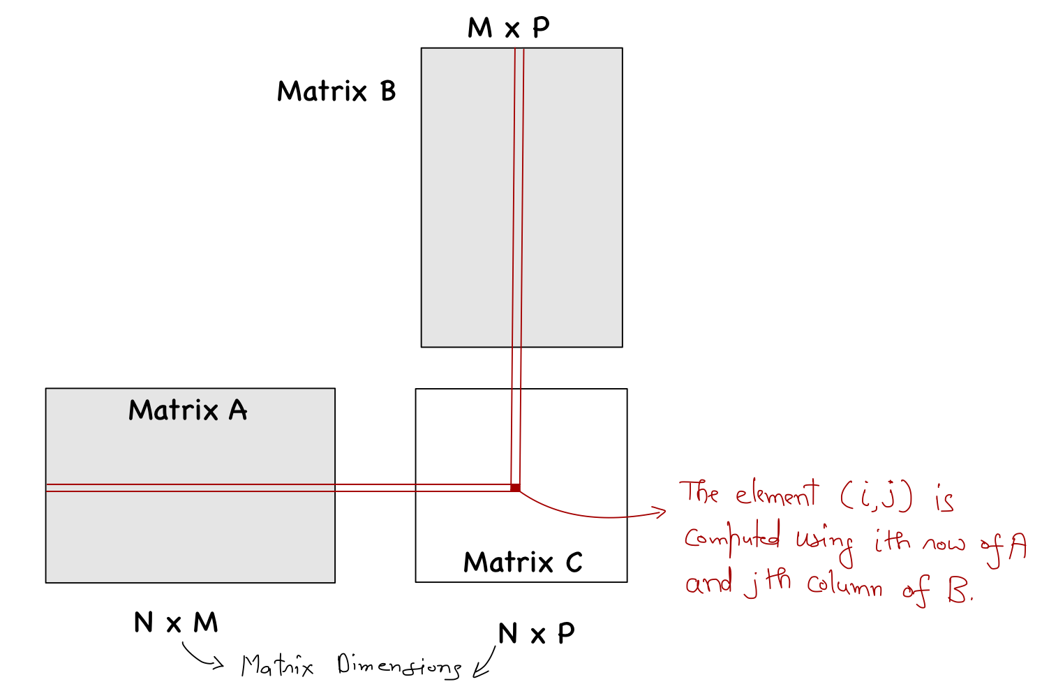
For simplicity, let's assume that \(N=M=P\). There are four main steps to sequential matrix multiplication:

1. Loop over every row of the matrix \(A\).
2. Loop over every column of the matrix \(B\).
3. Loop over all the elements in the selected row of \(A\) and column of \(B\). It is important to note that the number of elements in the two must be the same (that's essential for matrix multiplication to be valid).
4. Multiplication between the two elements is performed, and the result is added in every step.

void sq_mat_mul_cpu(float* A, float* B, float* C, int N)
{
    // 1. Loop over the rows
    for (int i = 0; i < N; i++)
    {
        // 2. Loop over the columns
        for (int j = 0; j < N; j++)
        {
            // Value at C[i,j]
            float value = 0;
            // 3. Loop over the elements
            for (int k = 0; k < N; k++)
            {
                // 4. Multiply and add 
                value += A[i*N+k] * B[k*N+j];
            }

            // Assigning calculated value back
            C[i*N+j] = value;
        }
    }
}

There are three loops in this algorithm and a total of \(N^2\) elements in matrix \(C\), where for each element, we need to perform around \(N\) multiplications and additions each. Hence, the total complexity is \(\approx N^2 \cdot (N+N) = \mathcal{O} (N^3)\). This means that with increasing \(N\), the computational cost increases drastically (cubic increase). However, if you analyze the algorithm carefully. You can see that the evaluation of the elements of the output matrix \(C\) does not depend on each other. In other words, we can execute the two loops (steps 1. and 2.) in parallel. GPUs are specially adapted to these types of computations (where \(N\) can be quite large) because the hardware contains 1000s of cores for parallel execution.

CPU vs GPU Hardware

CPUs and GPUs have execution units (called cores) that perform the arithmetic operations and an off-chip memory unit (RAM and VRAM, respectively) to store the required data. The big difference is that a CPU has much fewer cores than a GPU.

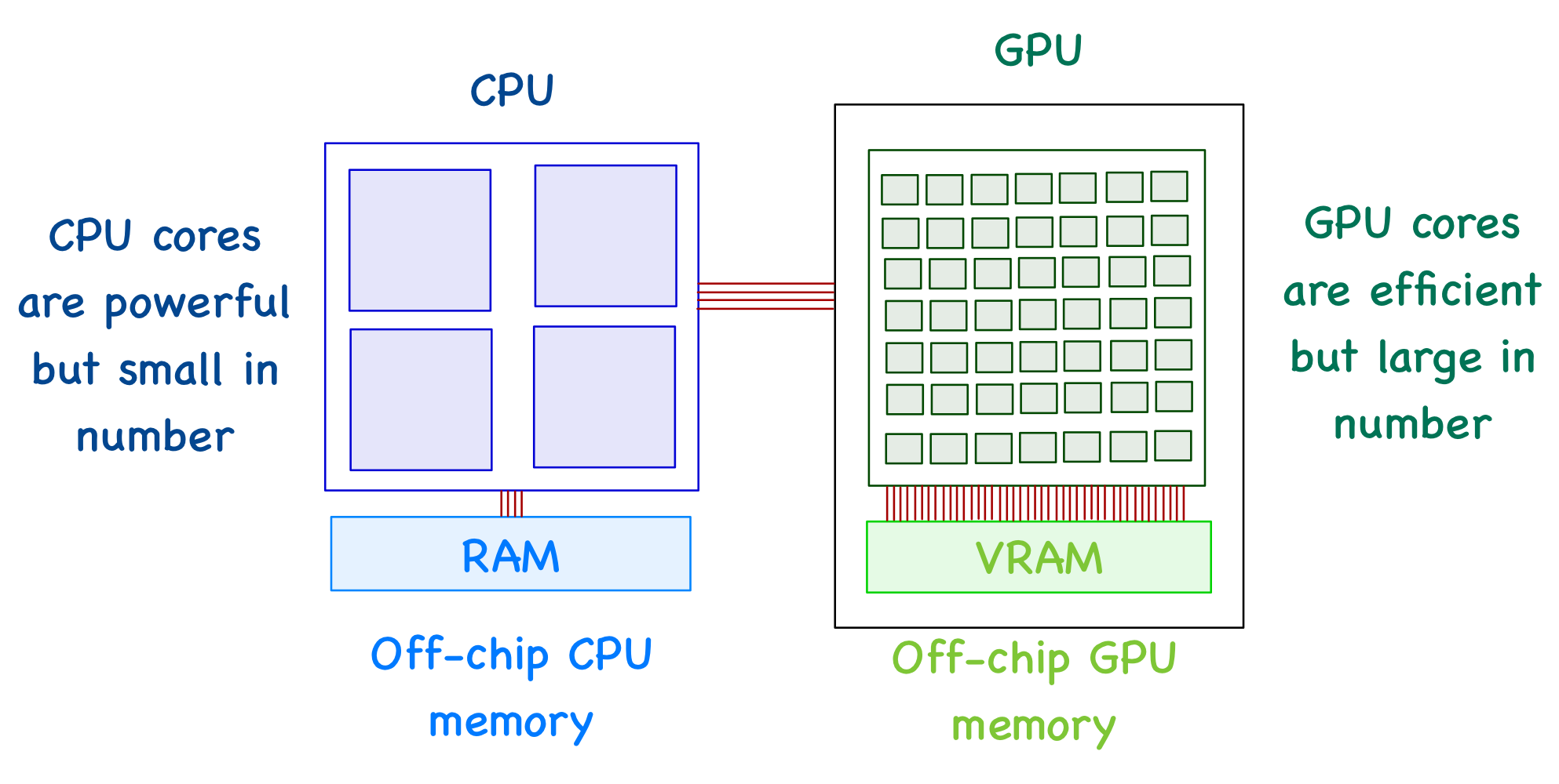
A GPU can't function independently. It's the job of a CPU to move data between RAM and VRAM. In other words, a CPU can be seen as an instructor who manages most of the tasks and is responsible for assigning specific tasks to the GPU (where it has an advantage).

Parallel Matrix Multiplication

CUDA is a heterogeneous computing platform developed by NVIDIA. CUDA C extends C programming language with minimal new syntax and library functions to allow programs to run on GPU and CPU cores. The structure of a CUDA C program reflects the presence of a CPU and one or more GPUs. It is such that the execution starts with the host, and the host assigns very specialized tasks to the device.

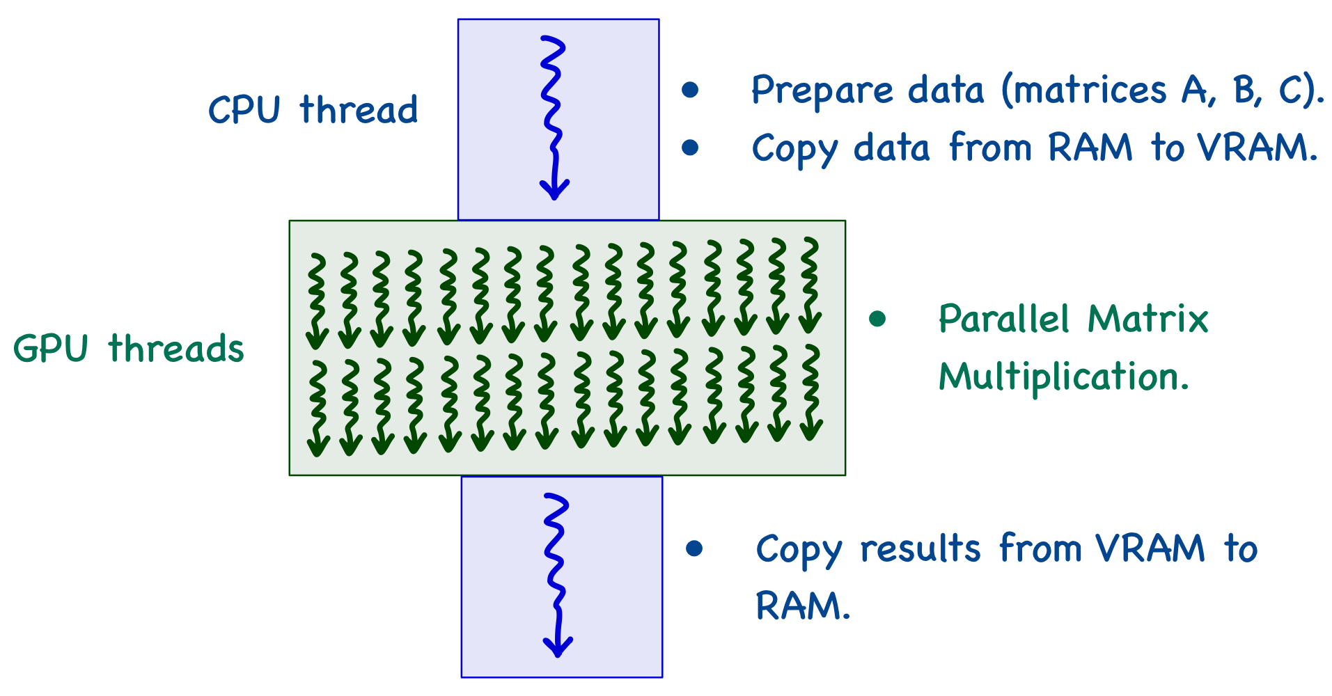
When the program starts, there is a single CPU thread that moves data from RAM to VRAM. It then calls a kernel function (which defines the executions to be performed on the GPU), and multiple threads are generated on the GPU. Each thread computes the same kernel function in parallel and stores the results in VRAM. The CPU thread then fetches the results from VRAM and puts it back into RAM, where the user can either print the results or perform further operations.

The very first step is to define matrices A and B. For simplicity, I'm only dealing with square matrices of size N, and dynamically allocating them (with elements assigned random values).

#include <stdio.h>
#include <stdlib.h>

#define MAX_NUM 10 
#define MIN_NUM -10 

int main(int argc, char const *argv[])
{
    // Generate NxN square matrices A and B
    int N = 100;
    float* A = (float*)malloc(N*N*sizeof(float));
    float* B = (float*)malloc(N*N*sizeof(float));
    for (int i = 0; i < N; i++)
    {
        for (int j = 0; j < N; j++)
        {
            A[i*N+j] = (float)(rand() % (MAX_NUM - MIN_NUM + 1) + MIN_NUM);
            B[i*N+j] = (float)(rand() % (MAX_NUM - MIN_NUM + 1) + MIN_NUM);
        }
    }
    
    return 0;
}

GPU Memory Allocation

Before copying matrices A and B from RAM to VRAM. Host code allocates memory for the three matrices on VRAM. It is done using cudaMalloc function (which is provided by CUDA). This function accepts two parameters:

• The first parameter is the address of the pointer variable for the select matrix. The address of this pointer must be cast to (void **) because the function expects a generic pointer (not restricted to a specific type).
• The second parameter is the size of the data to be allocated (in number of bytes).

// Device array pointers
float* d_A;
float* d_B;
float* d_C;

// Device memory allocation
cudaError_t err_A = cudaMalloc((void**) &d_A, N*N*sizeof(float));
CUDA_CHECK(err_A);

cudaError_t err_B = cudaMalloc((void**) &d_B, N*N*sizeof(float));
CUDA_CHECK(err_B);

cudaError_t err_C = cudaMalloc((void**) &d_C, N*N*sizeof(float));
CUDA_CHECK(err_C);

This allocates a specific amount of memory in VRAM and sets the pointer (whose address is passed as 1st parameter) to point at this memory location.

Data copy between RAM and VRAM

Once the memory has been allocated in the VRAM, data can be transferred from RAM using cudaMemcpy function. This function accepts four parameters:

• Pointer to the destination: When copying data from RAM to VRAM, this will be the device variable pointer (i.e., d_A or d_B).
• Pointer to the source: When copying data from RAM to VRAM, this will be the host variable pointer (i.e., A or B).
• Number of bytes to be copied.
• The direction of transfer: When copying data from RAM to VRAM, this will be cudaMemcpyHostToDevice. Note that this is a symbolic predefined constant of the CUDA programming environment.

// Copying A and B to device memory
cudaError_t err_A_ = cudaMemcpy(d_A, A, N*N*sizeof(float), cudaMemcpyHostToDevice);
CUDA_CHECK(err_A_);

cudaError_t err_B_ = cudaMemcpy(d_B, B, N*N*sizeof(float), cudaMemcpyHostToDevice);
CUDA_CHECK(err_B_);

Once the GPU has finished its execution, the results are stored in VRAM. The same function can be used to copy data from VRAM to RAM (by appropriately defining the function parameters).

// Copy back results
cudaError_t err_C_ = cudaMemcpy(C, d_C, N*N*sizeof(float), cudaMemcpyDeviceToHost);
CUDA_CHECK(err_C_);

Parallel Algorithm

The algorithm for parallel matrix multiplication (with square matrices of size N) is as follows:

1. \(N^2\) threads are generated on the GPU (one for each element of matrix \(C\)).
2. Each thread:
   1. Retrieves a row of matrix \(A\) and a column of matrix \(B\).
   2. Loops over the elements.
   3. Multiplies the two numbers and add the result to the total.

Thread Organization

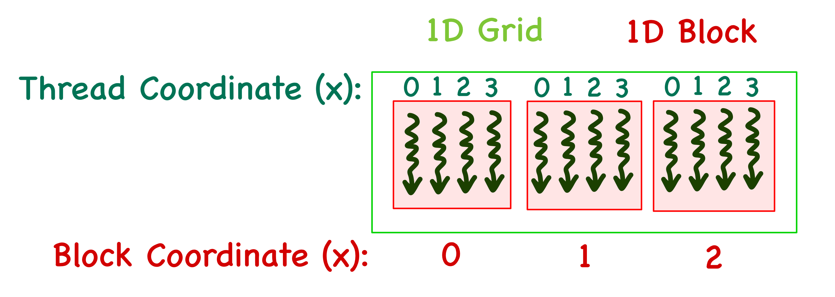
Now, who decides which thread works on which element of the matrix \(C\)? We need to understand how threads are organized on a GPU to answer this question. When the kernel function is called, it creates a grid of threads on the GPU. The grid is subdivided into multiple blocks, each containing the same amount of threads. The blocks in a grid and threads in a block can be arranged in a 1D/2D/3D manner with coordinates \(x,y,z\) assigned to the blocks and the threads inside each block.

• The 1D case is the simplest, with only an \(x\) index. For example, consider a grid with 3 blocks and 4 threads in each block. The blocks will then have \(x\) coordinates ranging from \(0\) to \(2\) and threads in each block will have \(x\) coordinates ranging from \(0\) to \(3\). It is important to note that the thread index is local for each block.

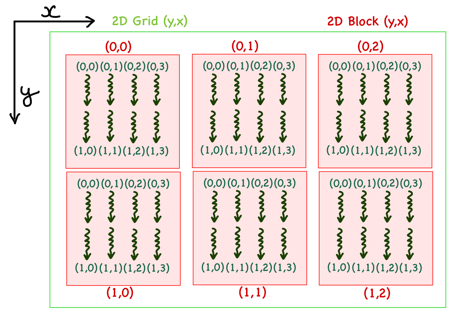
• In the 2D case, there are \(x\) and \(y\) indices. For example, consider a grid with 3 blocks in \(x\) direction and 2 blocks in \(y\) direction. Each block has 4 and 2 threads in \(x\) and \(y\) directions, respectively. In the case of a 2D organization, it is important to note that the \(y\) index precedes \(x\), i.e., it's written as \((y,x)\).

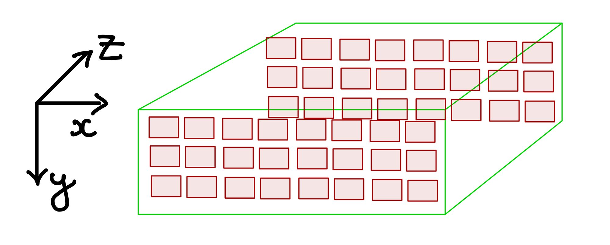
• For 3D, another dimension is added with the coordinates written as \((z,y,x)\).

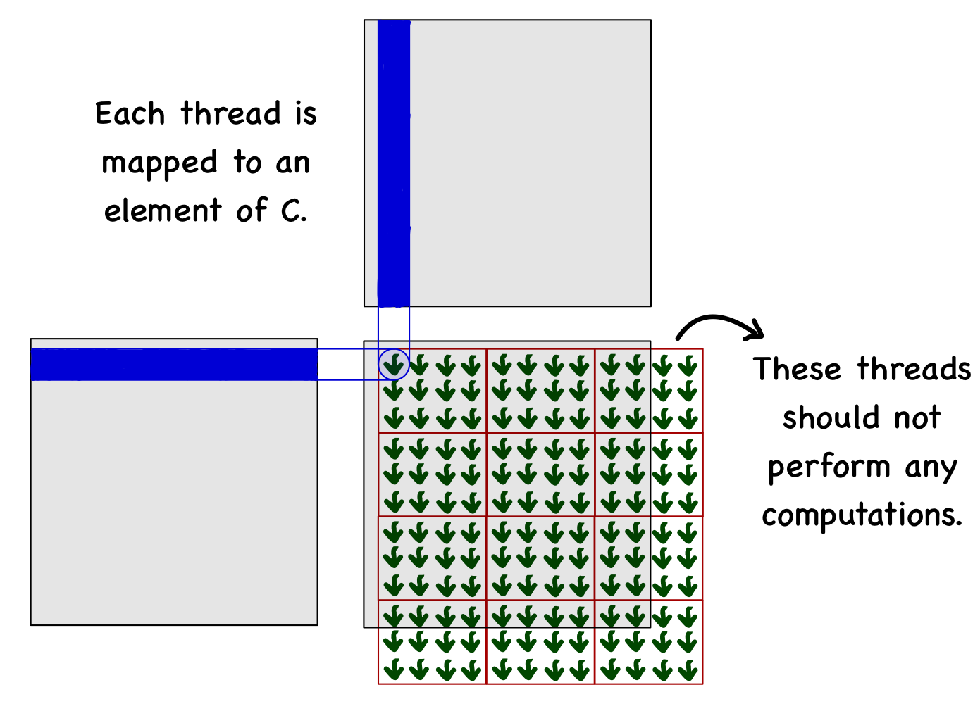
The data structure dictates whether 1D would be sufficient or 2D/3D organization is required. For matrices, it makes sense to use a 2D organization. Consider an example where A, B and C matrices are \(10 \times 10\). We decided to use the block size of \(3 \times 4\) (i.e., 3 threads in \(y\) and 4 threads in \(x\)). To cover all the elements of matrix C, we need 3 blocks in \(x\) direction and 4 blocks in \(y\) direction. Note that this will generate 12 threads each in \(x\) and \(y\) directions (more than elements in the matrix).

Kernel execution

The custom-defined CUDA type dim3 is used to define the details related to the grid and blocks:

• The number of threads in each block: dim3 dim_block(4, 3, 1). Note that in this case, the z dimension is set to 1.
• The number of blocks in the grid can then be decided based on the length of vectors and the total threads in each block: dim3 dim_grid(ceil(N/4.0), ceil(N/3.0), 1).

The kernel function sq_mat_mul_kernel defines the parallel matrix multiplication algorithm, executed by specifying the grid organization inside <<< >>> and passing the device variables.

sq_mat_mul_kernel<<<dim_grid, dim_block>>>(d_A, d_B, d_C, N);

An important thing to remember is that each thread executes the same kernel function. So, the first thing to do is identify the thread-to-element (of the matrix C) mapping, i.e., which element of C this thread will work on. It is done using CUDA variables:

• blockDim.x: Number of blocks in the grid in \(x\) direction.
• blockDim.y: Number of blocks in the grid in \(y\) direction. 
• blockIdx.x: \(x\) coordinate of the block to which this thread belongs.
• blockIdx.y: \(y\) coordinate of the block to which this thread belongs.
• threadIdx.x: \(x\) coordinate of the thread inside the specific block.
• threadIdx.y: \(y\) coordinate of the thread inside the specific block.

The next thing is to check whether this thread falls within the limits of the matrix (remember, two additional threads in each direction should not do anything). Finally, the thread will loop over the elements and perform the operations.

__global__ void sq_mat_mul_kernel(float* d_A, float* d_B, float* d_C, int N)
{
    // Identifying the thread mapping
    // Working on C[i,j]
    int i = blockDim.y*blockIdx.y + threadIdx.y;
    int j = blockDim.x*blockIdx.x + threadIdx.x;

    // Check the edge cases
    if (i < N && j < N)
    {
        // Value at C[i,j]
        float value = 0;
        // Loop over elements of the two vectors
        for (int k = 0; k < N; k++)
        {
            // Multiply and add
            value += A[i*N+k] * B[k*N+j];
        }

        // Assigning calculated value
        C[i*N+j] = value;
    }
}

Free GPU memory

At last, when everything is done, the device memory can be freed using cudaFree function.

// 7) Free device memory
cudaFree(d_A);
cudaFree(d_B);
cudaFree(d_C);

Conclusions

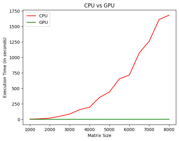
I compared the execution time for matrix multiplication on a CPU (Ryzen 7 7700) against a GPU (RTX 3090). The size of the matrices varied from 1000 to 8000, and the GPU provided a speedup of 2678% in the case of 8000!

You can check out the code repository using this link.

At the start of this blog post, I posed three questions. Let's summarize everything by answering those questions concisely.

• What is matrix multiplication?

Ans. Matrix multiplication is a binary operation in linear algebra that produces a new matrix from two input matrices.

• What is the computational complexity of matrix multiplication, and how can GPUs help reduce the computational cost?

Ans. The total complexity of matrix multiplication is \(\mathcal{O} (N^3)\). Upon carefully analyzing the algorithm, we can see that it can be parallelized effectively. GPUs are perfect for this because the hardware contains 1000s of cores for parallel execution.

• How can we use the CUDA programming model for a 2D dataset?

Ans. CUDA provides several API functions that can be used to define 2D grid and 2D blocks.

However, I didn't discuss how we should select the dimensions of the grid and blocks, i.e., the optimum number of blocks/threads in each dimension. To understand what impact thread organization has on the computational cost, we need an in-depth understanding of the GPU hardware. This is the topic for the next blog post.

References

1. Wen-Mei, W. Hwu, David B. Kirk, and Izzat El Hajj. Programming Massively Parallel Processors: A Hands-on Approach. Morgan Kaufmann, 2022.