Memory Coalescing and Tiled Matrix Multiplication
In this blog post, I first discuss how to transfer data from global memory efficiently and then show how shared memory can reduce global memory accesses and increase performance from 234 GFLOPS to 7490 GFLOPS.
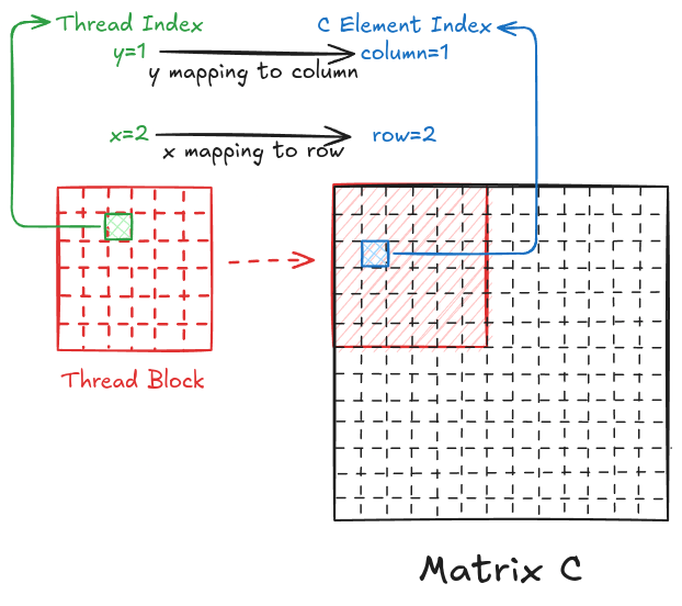
In Chapter 2, I ran a parallel matrix multiplication (on a GPU) and got a 2678x speedup from the sequential version (on a CPU) of the same problem. If you look at the code again (shown below), the thread-to-element mapping is such that the y index of the thread is mapped to the row of matrix C, and the x index of the thread is mapped to the column of matrix C.
__global__ void sq_mat_mul_kernel(float* d_A, float* d_B, float* d_C, int N)
{
    // Identifying the thread mapping
    // Working on C[i,j]
    int i = blockDim.y*blockIdx.y + threadIdx.y;
    int j = blockDim.x*blockIdx.x + threadIdx.x;

    // Check the edge cases
    if (i < N && j < N)
    {
        // Value at C[i,j]
        float value = 0;
        // Loop over elements of the two vectors
        for (int k = 0; k < N; k++)
        {
            // Multiply and add
            value += A[i*N+k] * B[k*N+j];
        }

        // Assigning calculated value
        C[i*N+j] = value;
    }
}
Code Snippet 1: CUDA C Square Matrix Multiplication Version 1

However, I can also map the y index of the thread to the column of matrix C and the x index of the thread to the row of matrix C.
__global__ void unco_sq_mat_mul_kernel(float* A, float* B, float* C, int N)
{
    // Working on C[i,j]
    int j = blockDim.y*blockIdx.y + threadIdx.y;
    int i = blockDim.x*blockIdx.x + threadIdx.x;

    // Parallel mat mul
    if (i < N && j < N)
    {
        // Value at C[i,j]
        float value = 0;
        for (int k = 0; k < N; k++)
        {
            value += A[i*N+k] * B[k*N+j];
        }

        // Assigning calculated value
        C[i*N+j] = value;
    }
}
Code Snippet 2: CUDA C Square Matrix Multiplication Version 2
I compared the runtime for the two implementations, and the former (Code Snippet 1 and Figure 1) ran 4.5x faster for the matrices of size 8000! To understand why this is happening, we must understand how global memory works and implement an important technique called Memory Coalescing.
Memory Coalescing
In Chapter 3, I mentioned that global memory has long latency and low bandwidth, which is usually a major bottleneck for most applications. This makes efficiently accessing data from global memory a top priority. To effectively utilize the global memory bandwidth, we must understand a few things about the architecture of the global memory. Global memory in CUDA devices is implemented using DRAM (Dynamic Random Access Memory) technology, which usually takes tens of nanoseconds to access a data byte. This starkly contrasts modern computing devices where the access speed is subnanosecond per byte. As the DRAM access speed is relatively slow, parallelism is used to increase the rate of data access (also known as memory access throughput).
Each time a DRAM location is accessed, a range of consecutive locations are also accessed in parallel. These consecutive location accesses and delivery are known as DRAM bursts. Current CUDA devices employ a technique that takes advantage of the fact that threads in a warp execute the same instruction at any given time. When all threads in a warp execute a load instruction, the hardware detects whether the memory accesses are consecutive or not. If they are consecutive, a lot of data can be transferred in parallel faster. In short, all threads in a warp must access consecutive global memory locations for optimum performance (this is known as coalesced access). Let's analyze the Code Snippets 1 and 2 in detail.
Figure 3 shows the pictorial analysis of Code Snippet 1. Consider the 0th warp, and each thread in this warp is responsible for evaluating the 1st 32 elements along the 0th row of matrix C. This means that each thread accesses the same row of matrix A and consecutive columns of matrix B. For any iteration k, threads in this warp access the consecutive elements of matrix B. That means all these 32 elements will be transferred in parallel at much higher speeds.
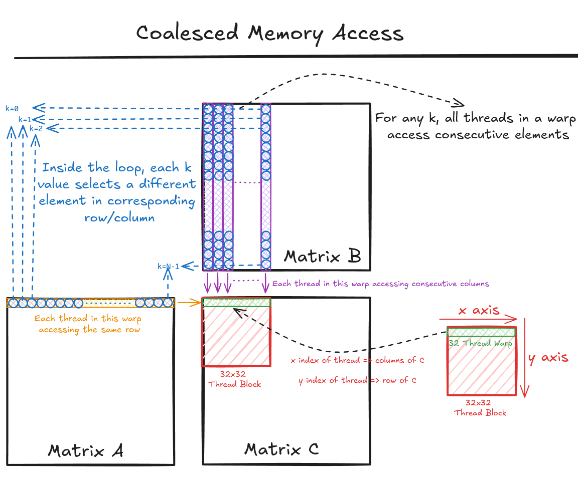
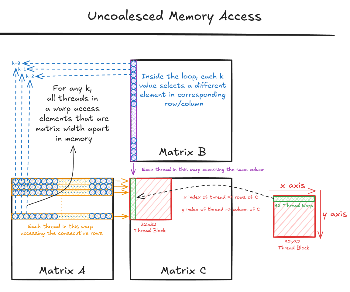
Figure 4 shows the pictorial analysis of Code Snippet 2. Consider the 0th warp, and each thread in this warp is responsible for evaluating the 1st 32 elements along the 0th column of matrix C. This means that each thread accesses the same column of matrix B and consecutive rows of matrix A. For any iteration k, threads in this warp access the elements of matrix A, which are N elements apart in the memory (remember that the 2D matrix is stored in a row-major layout in memory). As the threads in a warp are not accessing the consecutive elements in the memory, DRAM can not transfer these in parallel, hence requiring a separate load cycle for each element!
FLOPS Analysis
Keeping memory coalescing in mind, we must use the 1st implementation (Code Snippet 1). Now that the memory transfer is quite optimum, it would be interesting to analyze the kernel function and see how far off this implementation is from the theoretical limit (computational performance) on my GPU (RTX 3090). To recap, here is the parallel matrix multiplication kernel function with coalesced memory accesses.
__global__ void sq_mat_mul_kernel(float* d_A, float* d_B, float* d_C, int N)
{
    // Identifying the thread mapping
    // Working on C[i,j]
    int i = blockDim.y*blockIdx.y + threadIdx.y;
    int j = blockDim.x*blockIdx.x + threadIdx.x;

    // Check the edge cases
    if (i < N && j < N)
    {
        // Value at C[i,j]
        float value = 0;
        // Loop over elements of the two vectors
        for (int k = 0; k < N; k++)
        {
            // Multiply and add
            value += A[i*N+k] * B[k*N+j];
        }

        // Assigning calculated value
        C[i*N+j] = value;
    }
}
In the above code, the most important part (in terms of execution time) is the for loop that performs the dot product of a row of A and a column of B.
// Value at C[i,j]
float value = 0;
// Loop over elements of the two vectors
for (int k = 0; k < N; k++)
{
    // Multiply and add
    value += A[i*N+k] * B[k*N+j];
}

// Assigning calculated value
C[i*N+j] = value;
In every iteration of this loop, two global memory accesses (4 bytes each as its single precision float) are performed for one floating-point multiplication and one floating-point addition. Thus, the ratio of floating-point operations (FLOP) performed to bytes (B) accessed from global memory is 2/8=0.25 FLOP/B. This is also referred to as the computational intensity.
NVIDIA RTX 3090 has a peak memory bandwidth of 936.2 GB/s. It means that the GPU can transfer 936.2 GB of data from global memory to compute units in a second. As the kernel only performs 0.25 FLOP/B, the global memory bandwidth limits the kernel to 936.2 x 0.25=234.05 GFLOP per second (or GFLOPS). When I checked the GPU specifications, I found that RTX 3090 is capable of 35,580 GFLOPS! That means my version of parallel matrix multiplication uses just 0.65% of the maximum computing capacity!
Looking at the above analysis, the answer is clear. We must increase the number of operations performed per bytes accessed from the global memory. This is where we need to utilize the on-chip memory (as it's a high bandwidth and low latency memory unit). I have previously (in Chapter 3) discussed GPU architecture, and now, I will use that knowledge to increase the computational intensity of the code.
Parallel Matrix Multiplication
Standard Version
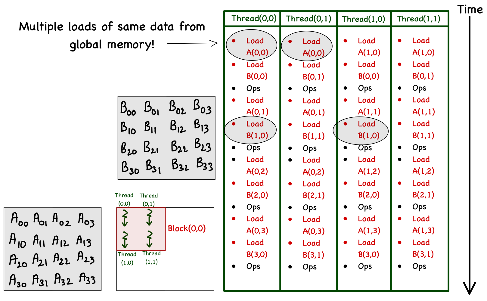
For simplicity, consider a matrix multiplication involving matrices of size 4. To facilitate parallel computations, define a 2 x 2 grid (i.e., 2 blocks each in x and y) and 2 x 2 blocks (i.e., 2 threads each in x and y). Focusing just on the computations involving block(0,0) (all the other blocks work exactly the same way), let's see how each thread in this block accesses data from the global memory. In the table below, I've listed the memory accesses (and operations) performed by each thread in this block. Each phase is a unit of time, and the order of operations (with respect to time) is from left to right, i.e., Phase 0 is followed by Phase 1, then Phase 2, and so on.
| Phase 0 | Phase 1 | Phase 2 | Phase 3 | |||||||||
| Thread[0,0] | Load A[0,0] | Load B[0,0] | C[0,0]+=A[0,0]*B[0,0] | Load A[0,1] | Load B[1,0] | C[0,0]+=A[0,1]*B[1,0] | Load A[0,2] | Load B[2,0] | C[0,0]+=A[0,2]*B[2,0] | Load A[0,3] | Load B[3,0] | C[0,0]+=A[0,3]*B[3,0] |
| Thread[0,1] | Load A[0,0] | Load B[0,1] | C[0,1]+=A[0,0]*B[0,1] | Load A[0,1] | Load B[1,1] | C[0,1]+=A[0,1]*B[1,1] | Load A[0,2] | Load B[2,1] | C[0,1]+=A[0,2]*B[2,1] | Load A[0,3] | Load B[3,1] | C[0,1]+=A[0,3]*B[3,1] |
| Thread[1,0] | Load A[1,0] | Load B[0,0] | C[1,0]+=A[1,0]*B[0,0] | Load A[1,1] | Load B[1,0] | C[1,0]+=A[1,1]*B[1,0] | Load A[1,2] | Load B[2,0] | C[1,0]+=A[1,2]*B[2,0] | Load A[1,3] | Load B[3,0] | C[1,0]+=A[1,3]*B[3,0] |
| Thread[1,1] | Load A[1,0] | Load B[0,1] | C[1,1]+=A[1,0]*B[0,1] | Load A[1,1] | Load B[1,1] | C[1,1]+=A[1,1]*B[1,1] | Load A[1,2] | Load B[2,1] | C[1,1]+=A[1,2]*B[2,1] | Load A[1,3] | Load B[3,1] | C[1,1]+=A[1,3]*B[3,1] |
Analyzing these memory accesses, we see they are quite inefficient! Just look at phase 0; Thread[0,0] and Thread [0,1] both access the same element A[0,0] from global memory. The same can be said for Thread[0,0] and Thread[1,0], where these two are again accessing B[1,0] individually from the global memory. These multiple global memory accesses are costly, and wouldn't it be better if we access these elements once, and then all threads in a block can use them whenever necessary? The answer is yes, and it can be done by utilizing the shared memory!
Tiled Version
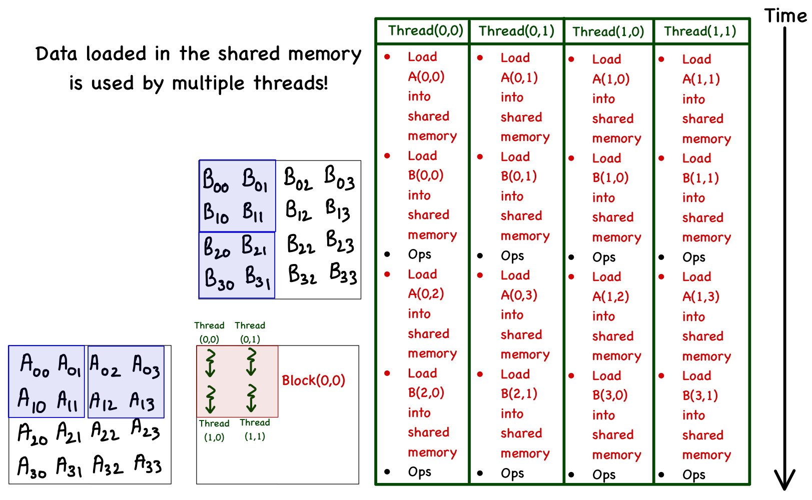
Shared memory allows us to store data temporarily and avoid multiple global memory accesses. There is a trade-off between using global memory and shared memory. Global memory is large but slow, and shared memory is fast but small. The strategy here is to partition the data into subsets called tiles so each tile fits into the shared memory.
In this example, the matrices A and B are partitioned into 2 x 2 tiles. Then, a tile is loaded so that each thread moves an element from global to shared memory (note that the block layout matches the tile layout). Once a tile is loaded, a partial dot product is performed. The program then moves on to the next tile and repeats the process. The complete dot product is achieved when all tiles are finished. The figure and the table below provide more details.
| Phase 0 | Phase 1 | |||||
| Global Memory to Shared Memory | Global Memory to Shared Memory | |||||
| Thread[0,0] | Load A[0,0] -> sh_A[0,0] | Load B[0,0] -> sh_B[0,0] | C[0,0]+=sh_A[0,0]*sh_B[0,0] + sh_A[0,1]*sh_B[1,0] | Load A[0,2] -> sh_A[0,2] | Load B[2,0] -> sh_B[2,0] | C[0,0]+=sh_A[0,2]*sh_B[2,0] + sh_A[0,3]*sh_B[3,0] |
| Thread[0,1] | Load A[0,1] -> sh_A[0,1] | Load B[0,1] -> sh_B[0,1] | C[0,1]+=A[0,0]*B[0,1] + sh_A[0,1]*sh_B[1,1] | Load A[0,3] -> sh_A[0,3] | Load B[2,1] -> sh_B[2,1] | C[0,1]+=A[0,2]*B[2,1] + sh_A[0,3]*sh_B[3,1] |
| Thread[1,0] | Load A[1,0] -> sh_A[1,0] | Load B[1,0] -> sh_B[1,0] | C[1,0]+=sh_A[1,0]*sh_B[0,0] + sh_A[1,1]*sh_B[1,0] | Load A[1,2] -> sh_A[1,2] | Load B[3,0] -> sh_B[3,0] | C[1,0]+=sh_A[1,2]*sh_B[2,0] + sh_A[1,3]*sh_B[3,0] |
| Thread[1,1] | Load A[1,1] -> sh_A[1,1] | Load B[1,1] -> sh_B[1,1] | C[1,1]+=sh_A[1,0]*sh_B[0,1]+sh_A[1,1]*sh_B[1,1] | Load A[1,3] -> sh_A[1,3] | Load B[3,1] -> sh_B[3,1] | C[1,1]+=sh_A[1,2]*sh_B[2,1]+sh_A[1,3]*sh_B[3,1] |
The big change in the matrix multiplication using shared memory is that the total number of load operations is halved! You can see this as we now only have two phases, and in each phase, two sets of multiplications and additions are performed. It is also important to note that all this is possible only because the threads in a block can access the same shared memory!
Writing a kernel function that supports tiling can be a little tricky. However, I will explain everything by dividing them into 8 simple steps:
- The very first thing we need to do is make sure that the dimensions of the block are the same as the tile size and that the size of the matrix is fully divisible by the tile size.
// Ensure that TILE_WIDTH = BLOCK_SIZE
assert(TILE_WIDTH == blockDim.x);
assert(TILE_WIDTH == blockDim.y);

// Ensure N%TILE_WIDTH == 0
assert(N % TILE_WIDTH == 0);- Let's store the block and thread indices in variables and find out the coordinate of the element of C that the select thread will work on. Then, we can also allocate shared memory for tiles of matrices A and B.
// Details regarding this thread
int by = blockIdx.y;
int bx = blockIdx.x;

int ty = threadIdx.y;
int tx = threadIdx.x;

// Working on C[i,j]
int i = TILE_WIDTH*by + ty;
int j = TILE_WIDTH*bx + tx;

// Allocating shared memory
__shared__ float sh_A[TILE_WIDTH][TILE_WIDTH];
__shared__ float sh_B[TILE_WIDTH][TILE_WIDTH];- Next, we divide matrices A and B into multiple tiles and loop over the tiles one by one (I call each loop iteration a phase).
// Parallel mat mul
float value = 0;
// Looping over the tiles
for (int phase = 0; phase < N/TILE_WIDTH; phase++)
{
    // .
    // .
    // .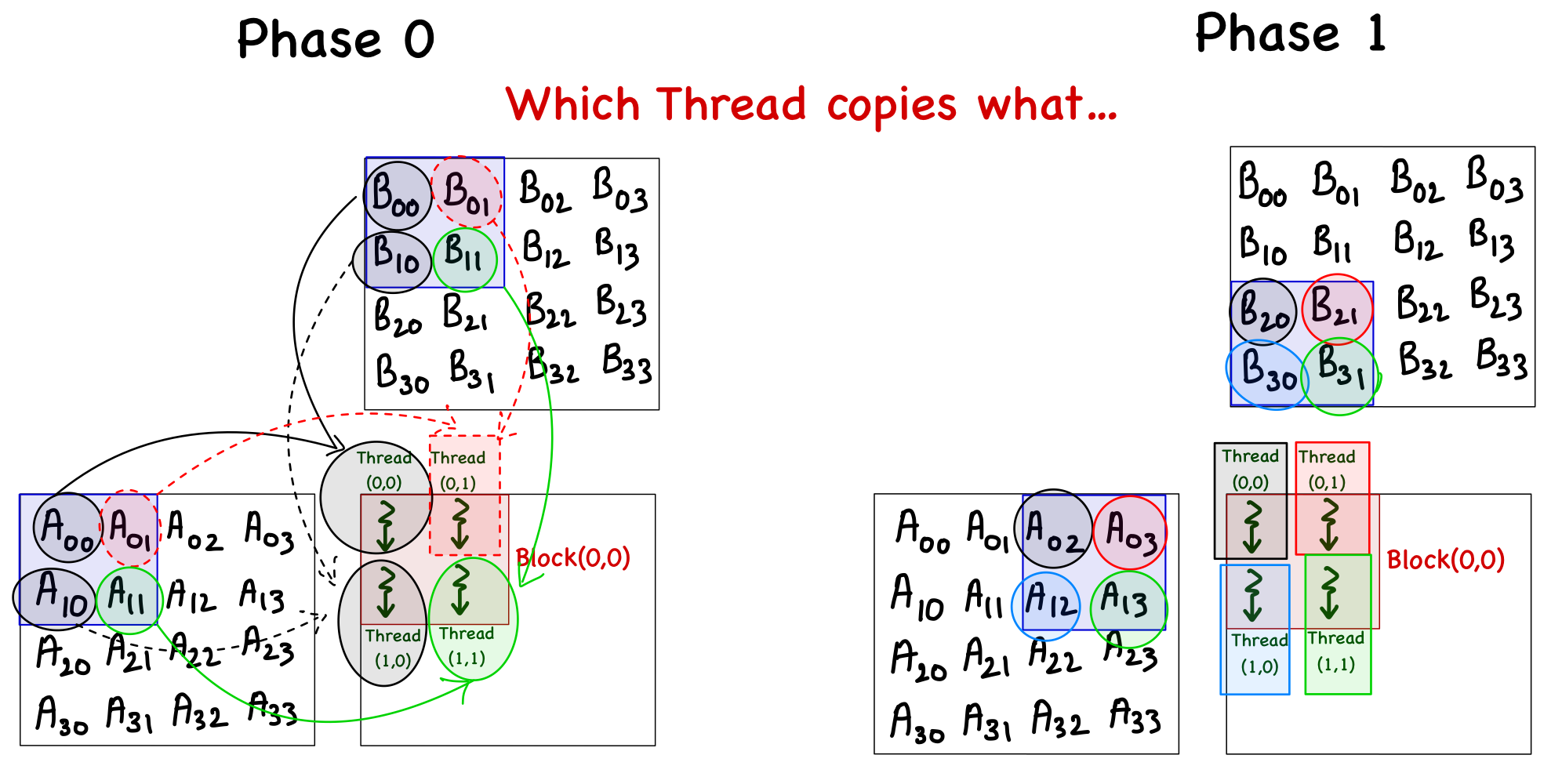
}- As the block size is the same as the tile width, each thread is responsible for copying an element from matrices A and B. The figure below illustrates which thread will copy which element, but here are the key points:
- For an element of matrix A, the row index is the same as the global index of the thread in the y direction (i.e.,
i), and the column index is decoded by first deciding which tile number it is (i.e.phase*TILE_WIDTH), and then the local thread index in the x direction (i.e.tx) is added to it (remember that the x index of the thread maps to the columns of A). - For an element of matrix B, the row index is decoded by first deciding which tile number it is (i.e.
phase*TILE_WIDTH), and then the local thread index in the y direction (i.e.ty) is added to it (remember that the y index of the thread maps to the rows of B), and the column index is the same as the global index of the thread in the x direction (i.e.,j).
- For an element of matrix A, the row index is the same as the global index of the thread in the y direction (i.e.,
// Parallel mat mul
float value = 0;
for (int phase = 0; phase < N/TILE_WIDTH; phase++)
{
    // Load Tiles into shared memory
    sh_A[ty][tx] = A[(i)*N + phase*TILE_WIDTH+tx];
    sh_B[ty][tx] = B[(phase*TILE_WIDTH + ty)*N+j];

    // .
    // .
    // .
}- The whole point of tiling is that all threads in a block can access all elements (necessary) for their computations. As data copying into shared memory is done in parallel by multiple threads (and it's coalesced), we must ensure the complete tile is loaded before moving forward! This is done using
__syncthreads()which basically holds the code execution (at this point) until all threads have reached there.
// Parallel mat mul
float value = 0;
for (int phase = 0; phase < N/TILE_WIDTH; phase++)
{
    // Load Tiles into shared memory
    sh_A[ty][tx] = A[(i)*N + phase*TILE_WIDTH+tx];
    sh_B[ty][tx] = B[(phase*TILE_WIDTH + ty)*N+j];
    __syncthreads();

    // .
    // .
    // .
}- Finally, we can perform the dot product using the data loaded into the shared memory.
// Parallel mat mul
float value = 0;
for (int phase = 0; phase < N/TILE_WIDTH; phase++)
{
    // Load Tiles into shared memory
    sh_A[ty][tx] = A[(i)*N + phase*TILE_WIDTH+tx];
    sh_B[ty][tx] = B[(phase*TILE_WIDTH + ty)*N+j];
    __syncthreads();

    // Dot product
    for (int k = 0; k < TILE_WIDTH; k++)
        value += sh_A[ty][k] * sh_B[k][tx];

    // .
    // .
    // .
}- As the loop moves to the next iteration, it starts by loading the shared memory with new tiles. For this reason, we must again ensure that all threads have completed their dot product evaluation and avoid data corruption!
// Parallel mat mul
float value = 0;
for (int phase = 0; phase < N/TILE_WIDTH; phase++)
{
    // Load Tiles into shared memory
    sh_A[ty][tx] = A[(i)*N + phase*TILE_WIDTH+tx];
    sh_B[ty][tx] = B[(phase*TILE_WIDTH + ty)*N+j];
    __syncthreads();

    // Dot product
    for (int k = 0; k < TILE_WIDTH; k++)
        value += sh_A[ty][k] * sh_B[k][tx];
    __syncthreads();
}- The last step is to store the calculated value in matrix C.
// Assigning calculated value
C[i*N+j] = value;
Putting all 8 steps together, we have a parallel implementation of tiled matrix multiplication.
__global__ void tiled_sq_mat_mul_kernel(float* A, float* B, float* C, int N)
{
    // Ensure that TILE_WIDTH = BLOCK_SIZE
    assert(TILE_WIDTH == blockDim.x);
    assert(TILE_WIDTH == blockDim.y);

    // Ensure N%TILE_WIDTH == 0
    assert(N % TILE_WIDTH == 0);

    // Details regarding this thread
    int by = blockIdx.y;
    int bx = blockIdx.x;

    int ty = threadIdx.y;
    int tx = threadIdx.x;

    // Working on C[i,j]
    int i = TILE_WIDTH*by + ty;
    int j = TILE_WIDTH*bx + tx;

    // Allocating shared memory
    __shared__ float sh_A[TILE_WIDTH][TILE_WIDTH];
    __shared__ float sh_B[TILE_WIDTH][TILE_WIDTH];

    // Parallel mat mul
    float value = 0;
    for (int phase = 0; phase < N/TILE_WIDTH; phase++)
    {
        // Load Tiles into shared memory
        sh_A[ty][tx] = A[(i)*N + phase*TILE_WIDTH+tx];
        sh_B[ty][tx] = B[(phase*TILE_WIDTH + ty)*N+j];
        __syncthreads();

        // Dot product
        for (int k = 0; k < TILE_WIDTH; k++)
            value += sh_A[ty][k] * sh_B[k][tx];
        __syncthreads();
    }
    // Assigning calculated value
    C[i*N+j] = value;
}
In the above code, there are two big assumptions:
- Matrices are square.
- Matrix size is fully divisible by the tile size.
Let's now see how to improve the code by removing these restrictions.
General Matrix Multiplication (Tiled)
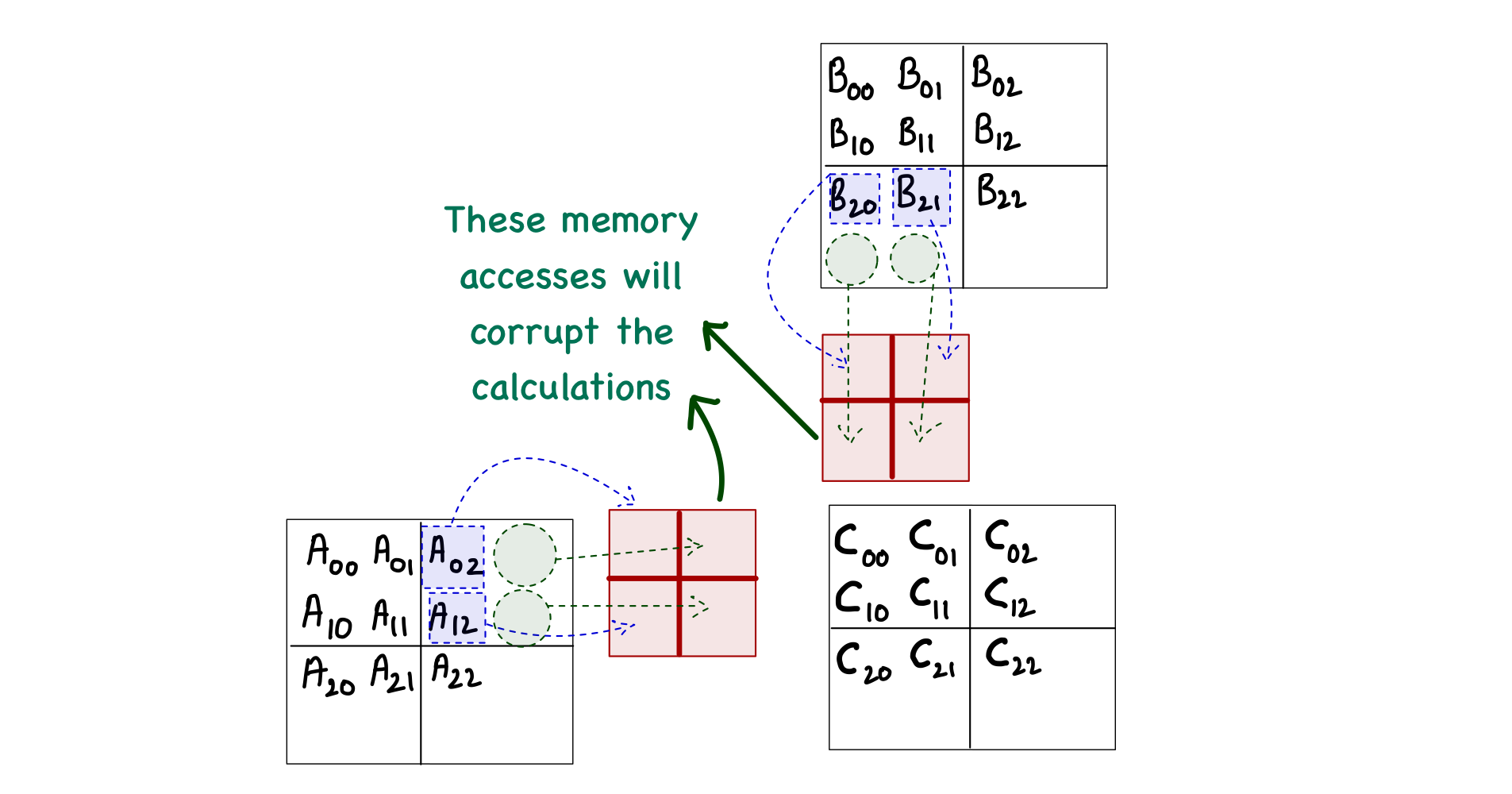
Starting with the case when the matrix size is not fully divisible by the tile size. Consider a matrix multiplication involving 3 x 3 matrices (and the tile size is 2). One problem in this case would arise during phase 1 of computing the block[0,0], when the threads will attempt to load elements \(A_{0,2}\), \(A_{1,2}\), \(B_{2,0}\), and \(B_{2,1}\).
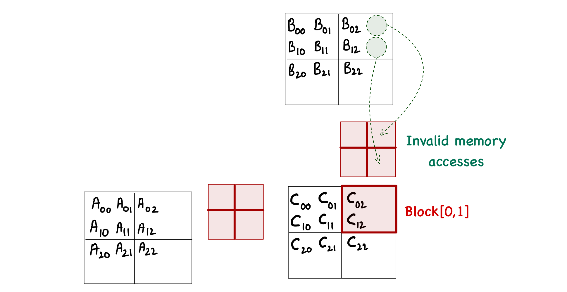
With this much analysis, you might think that this problem only occurs during the last phase of calculations. However, this is not true. When computing block[0,1], we can see the invalid memory accesses during phase 0 as well!
Another thought might occur to simply exclude the threads that are outside the bounds of matrix C. This is also untrue, as the thread[0,1] in block[1,1] is not computing any C element but will load \(A_{2,1}\) during phase 0.
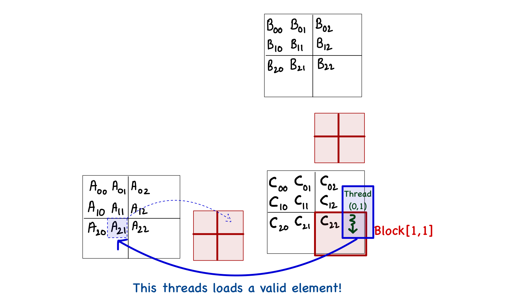
The only solution for this problem is to individually check the validity of every element of A and B during the load into the shared memory and then perform another check when storing the result back into matrix C. This can be done fairly easily in code as we already know what values indicate the x and y indices of any element of A and B. One thing to remember is that if a thread does not load a value into shared memory, then that spot in the shared memory must be set to 0 to avoid corruption of the final results. The resulting kernel function is as follows.
__global__ void tiled_sq_mat_mul_kernel(float* A, float* B, float* C, int N)
{
    // Ensure that TILE_WIDTH = BLOCK_SIZE
    assert(TILE_WIDTH == blockDim.x);
    assert(TILE_WIDTH == blockDim.y);

    // Details regarding this thread
    int by = blockIdx.y;
    int bx = blockIdx.x;

    int ty = threadIdx.y;
    int tx = threadIdx.x;

    // Working on C[i,j]
    int i = TILE_WIDTH*by + ty;
    int j = TILE_WIDTH*bx + tx;

    // Allocating shared memory
    __shared__ float sh_A[TILE_WIDTH][TILE_WIDTH];
    __shared__ float sh_B[TILE_WIDTH][TILE_WIDTH];

    // Parallel mat mul
    float value = 0;
    for (int phase = 0; phase < ceil((float)N/TILE_WIDTH); phase++) // Ceiling function to ensure that extra phase at the boundary
    {
        // Load Tiles into shared memory by checking locations
        if ((i < N) && ((phase*TILE_WIDTH+tx) < N))
          sh_A[ty][tx] = A[(i)*N + phase*TILE_WIDTH+tx];
        else
          sh_A[ty][tx] = 0.0f;

        if (((phase*TILE_WIDTH + ty) < N) && (j < N))
          sh_B[ty][tx] = B[(phase*TILE_WIDTH + ty)*N+j];
        else
          sh_B[ty][tx] = 0.0f;
        __syncthreads();

        // Dot product
        for (int k = 0; k < TILE_WIDTH; k++)
            value += sh_A[ty][k] * sh_B[k][tx];
        __syncthreads();
    }
    // Assigning calculated value by checking location
    if ((i < N) && (j < N))
      C[i*N+j] = value;
}
Finally, accommodating rectangular matrices is an easy modification. The kernel function will accept three integers representing the dimension of the three matrices (details shown in figure below), and then we replace N with those values appropriately (as shown in the code snippet below).
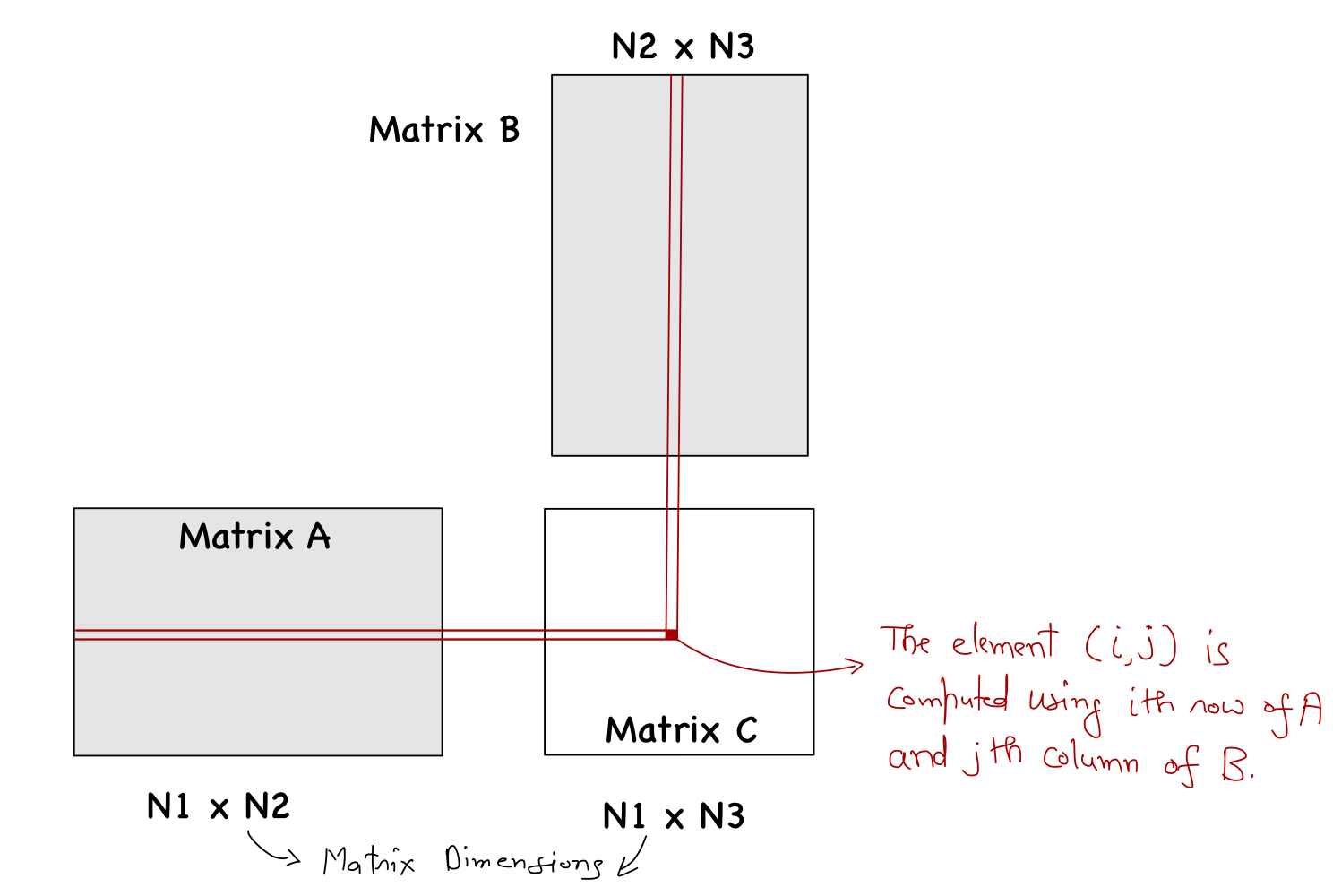
__global__ void tiled_mat_mul_kernel(float* A, float* B, float* C, int N1, int N2, int N3)
{
    // Ensure that TILE_WIDTH = BLOCK_SIZE
    assert(TILE_WIDTH == blockDim.x);
    assert(TILE_WIDTH == blockDim.y);

    // Details regarding this thread
    int by = blockIdx.y;
    int bx = blockIdx.x;

    int ty = threadIdx.y;
    int tx = threadIdx.x;

    // Working on C[i,j]
    int i = TILE_WIDTH*by + ty;
    int j = TILE_WIDTH*bx + tx;

    // Allocating shared memory
    __shared__ float sh_A[TILE_WIDTH][TILE_WIDTH];
    __shared__ float sh_B[TILE_WIDTH][TILE_WIDTH];

    // Parallel mat mul
    float value = 0;
    for (int phase = 0; phase < ceil((float)N2/TILE_WIDTH); phase++)
    {
        // Load Tiles into shared memory
        if ((i < N1) && ((phase*TILE_WIDTH+tx) < N2))
          sh_A[ty][tx] = A[(i)*N2 + phase*TILE_WIDTH+tx];
        else
          sh_A[ty][tx] = 0.0f;

        if (((phase*TILE_WIDTH + ty) < N2) && (j < N3))
          sh_B[ty][tx] = B[(phase*TILE_WIDTH + ty)*N3+j];
        else
          sh_B[ty][tx] = 0.0f;
        __syncthreads();

        // Dot product
        for (int k = 0; k < TILE_WIDTH; k++)
            value += sh_A[ty][k] * sh_B[k][tx];
        __syncthreads();
    }
    // Assigning calculated value
    if ((i < N1) && (j < N3))
      C[i*N3+j] = value;
}
Optimum Tile Size
Different GPUs have different shared memory sizes. In my case (RTX 3090), available shared memory per block is 49152 Bytes. From the kernel function, we can see that shared memory in each block holds tiles of A and B, which results in a total of 2 x TILE_WIDTH x TILE_WIDTH x 4 Bytes. Generally speaking, a larger tile size is preferred. However, CUDA also restricts a maximum of 1024 threads per block, and as the tile size is the same as the block dimensions, the best we can do is a 32 x 32 tile!
For 32 x 32 tiles, the global memory accesses are reduced by a factor of 32! This means that the ratio of floating-point operations (FLOP) performed to bytes (B) accessed from global memory has increased to (2 x 32)/8=8 FLOP/B. For the NVIDIA RTX 3090, which has a peak memory bandwidth of 936.2 GB/s, the global memory bandwidth limits the kernel to 936.2 x 8 = 7489.6 GFLOPS. This is 21% of the maximum 35,580 GFLOPS that RTX 3090 can do. That's a big jump from 0.65% in the case of matrix multiplication without tiles.
Conclusion
In summary,
- Global memory transfer is the biggest bottleneck. Hence, we must ensure coalesced memory accesses to maximize the throughput.
- The memory speed severely limits the execution speed. Hence, to achieve good performance, we must write algorithms that perform many operations for every byte of memory accessed.
- Tiling provides a way to utilize the on-chip memory effectively, which can reduce the execution speed significantly.
- On-chip memory units are small in size. Hence, the programmer should write code keeping this fact in mind.