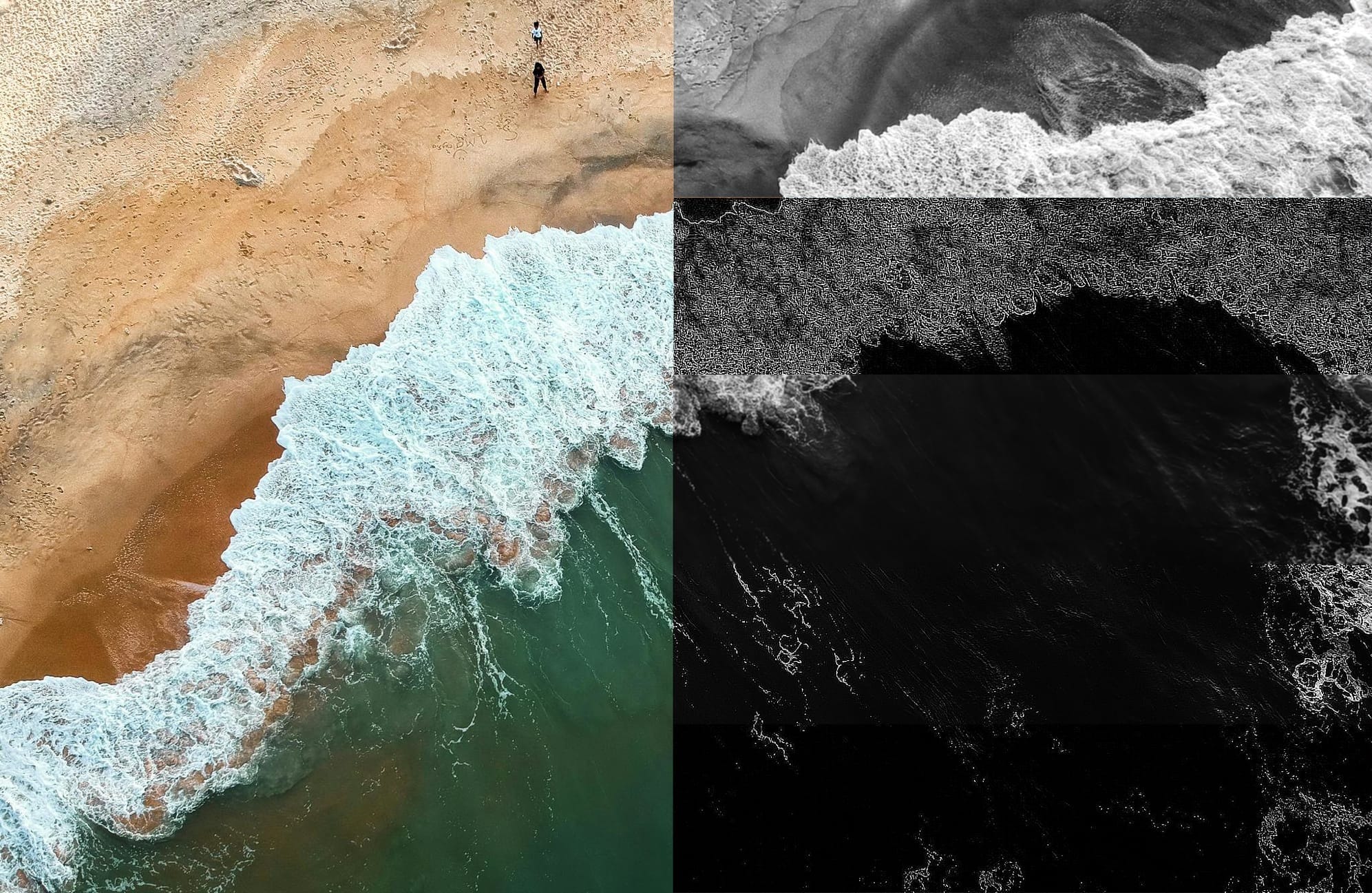
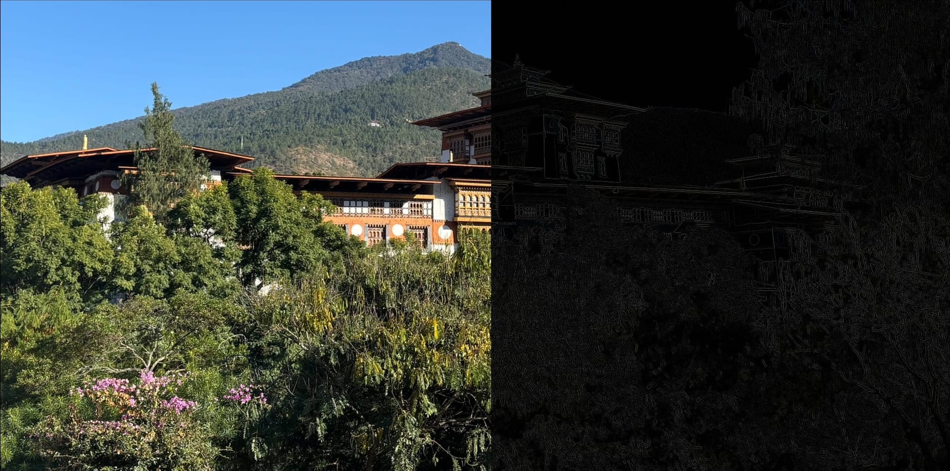
A while ago, I was going through the pics from my last vacation, casually editing using the built-in filters in the Photos app, and I never really paid attention before that the whole process is quite snappy. This led me to think about whether I could build something similar. Apple or Google conducts extensive research in image processing; I cannot match that. Image processing is not my expertise, and I want to keep things simple. Then I remembered a neat little algorithm (from my undergrad days) called convolution.

This mini-project is all about applying filters to high-resolution images using convolution and accelerating the whole process using a GPU. I will show how you can apply five different filters (see Figure 0.1) using a single algorithm and, at the same time, improve the application runtime by \(11\text{x}\) using a GPU (compared to a basic CPU implementation).

Convolution

Convolution is an array operation in which each output element is a weighted sum of the corresponding input elements and a collection of several neighboring elements (symmetric around the location being computed). The weights used in the calculations are defined by a filter array known as a convolution filter or simply filter. The size of the filter is an odd number \((2r+1)\), such that the weighted sum calculation is symmetric around the element being calculated. Convolutions can be 1D, 2D or 3D.

Consider an example involving 1D convolution where the input array is of length \(5\) and filter of size \(3\) (i.e., radius \(1\)). Figure 0.2 shows how the convolution is applied in this case. An important thing to note is how the 1st and last element is computed. Boundary conditions naturally arise here, and the missing input elements (there is just one in this case) are set to \(0\). These missing input elements are referred to as ghost cells.

2D convolution works exactly the same, but the input array and filter are both 2D. Figure 0.3 shows 2D convolution on a \(5 \times 5\) input image using \(3 \times 3\) filter.

CPU Implementation

Sequential implementation using a CPU is pretty straightforward. The function cpu_conv2d accepts input image N, filter matrix F, output image P, filter radius r, and the input/output image dimensions (n_rows and n_cols).

/*
Input Image: N
Filter: F
Output Image: P
Filter Radius: r
Num of rows in input/output image: n_rows
Num of cols in input/output image: n_cols
*/
void cpu_conv2d(float *N, float *F, float *P, int r, int n_rows, int n_cols)
{
    
}

The strategy to perform 2D convolution can be summed up as follows (with the complete code shown in Figure 0.4):

1. Loop over each output element. For each output element:
   1. Loop over the elements of the filter matrix.
   2. Figure out filter to input element mapping.
   3. Check for ghost cells and perform the calculations involving input and filter elements.

/*
Input Image: N
Filter: F
Output Image: P
Filter Radius: r
Num of rows in input/output image: n_rows
Num of cols in input/output image: n_cols
*/
void cpu_conv2d(float *N, float *F, float *P, int r, int n_rows, int n_cols)
{
    // 1. Loop over elements of output matrix P
    for (int out_col = 0; out_col < n_rows; out_col++)
    {
        for (int out_row = 0; out_row < n_cols; out_row++)
        {
            // Output in the register
            float p_val = 0.0f;

            // 1a. Loop over elements of the filter F
            for (int f_row = 0; f_row < 2*r+1; f_row++)
            {
                for (int f_col = 0; f_col < 2*r+1; f_col++)
                {
                    // 1b. Input-filter mapping
                    int in_row = out_row + (f_row - r);
                    int in_col = out_col + (f_col - r);

                    // 1c. Ignore computations involving ghost cells
                    if ((in_row >= 0 && in_row < n_rows) && (in_col >= 0 && in_col < n_cols))
                        p_val += F[f_row*(2*r+1) + f_col] * N[in_row*n_cols + in_col];
                }   
            }
            // Update value in the output matrix
            P[out_row*n_cols + out_col] = p_val;   
        }   
    }
}

Benchmarking

For an image of size \(2048 \times 2048\), it took \(0.060\) seconds to apply a \(3 \times 3\) filter using my CPU (AMD Ryzen™ 7 7700). While this is not too bad, it amounts to around \(16\) frames per second (FPS). On a live video feed, where \(24\) FPS (or even \(60\) FPS) is normal, this might not be good enough.

Conclusion

This three-part blog post series discusses how to accelerate convolution using a GPU and achieve over \(100\) FPS performance. Specifically, I will be discussing:

1. Naive GPU implementation using CUDA C++.
2. Using constant memory to store filter matrix and tiling to reduce global memory accesses.
3. Using pinned global memory to speed up data transfer between CPU and GPU memory.

References

1. Kirk, David B., and W. Hwu Wen-Mei. Programming massively parallel processors: a hands-on approach. Morgan kaufmann, 2016.
2. Ansorge, Richard. Programming in parallel with CUDA: a practical guide. Cambridge University Press, 2022.