Mini Project: 3D Earthquake Simulation
This blog post explains how I developed a 3D earthquake wave simulation in C++. The simulation models seismic waves emanating from an earthquake, propagating through the Earth's crust, and reaching the surface.

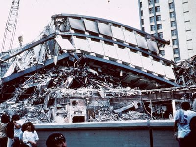
Earthquakes are unpredictable and can be extremely dangerous. Knowing how the surface will respond in an earthquake is extremely important if we want to protect our infrastructure. The intensity at the surface depends heavily on the type of soil. Hard soils or rocks provide a more stable foundation than soft soils like soft clay, where the ground motion can be amplified significantly. This happened in Mexico City's 1985 earthquake, where soft clay amplified ground motion by over 20x!
This blog post will explain how I developed a 3D earthquake wave simulation in C++. The simulation models seismic waves emanating from an earthquake, propagating through the Earth's crust, and reaching the surface.
Chapter 1: The Wave Equation
Partial differential equations (PDEs) are fundamental mathematical tools that capture and analyze diverse physical phenomena, including earthquakes. In the context of earthquake dynamics, the wave equation (equation 1.1) governs the evolution of the displacement field \(u(x,y,z,t)\), which arises from an energy release represented by the source term \(s(x,y,z,t)\). The medium properties, such as wave propagation speed \(c(x,y,z)\), further define the system’s behavior. Simulating earthquakes fundamentally involves solving this PDE numerically. The displacement field’s spatiotemporal evolution—dictated by the interplay of the source term \(s(x,y,z,t)\), wave speed distribution \(c(x,y,z)\), and boundary conditions—enables the visualization and quantification of the earthquake effects.

The whole process starts with the source that releases the energy. To mimic an earthquake, I needed the source to be instantaneous and highly localized. Derivative of a Gaussian (shown in equation 1.2) was an ideal choice because it was easy to control the nature of the energy released using two parameters, \(f_0\) and \(t_0\). Large \(f_0\) made the source instantaneous, and \(t_0\) controlled the distribution of the released energy with time (see Figure 1.1).

Figure 1.1: Derivative of Gaussian as a source function.
To make the source (defined in equation 1.2) localized, I multiplied it with the delta functions. Equation 1.3 shows the definition of the localized source function, where the term \(\delta(x,x_s) \cdot \delta(y,y_s) \cdot \delta(z,z_s)\) is zero everywhere, except at \(x=x_s, y=y_s, z=z_s\).

The wave equation (without the source term) essentially expresses Newton's Second Law (\(F = ma\)) for a continuous medium. It states that the acceleration of any point on the wave is proportional to the curvature at that point. This second-order nature of the wave equation allows it to describe oscillatory behavior, where energy continuously transfers between potential energy (related to displacement \(u\)) and kinetic energy (related to velocity \(c\)), resulting in wave propagation. The term \(c(x,y,z)\) represents the medium velocity. In simple terms, this dictates the speed of the wave propagation. Interesting things happen when the wave encounters a sharp change in the medium velocity. For example, in Figure 1.2, a part of the wave reflects at the sea-Earth interface.
Figure 1.2: Earthquake wave propagation in a relatively simple subsurface model.
Chapter 2: Building the Simulator
I used the finite-difference method to solve the wave equation numerically. Let's start with the 1D wave equation (shown in equation 2.1). I'm doing this because it's easy to understand the concepts in 1D and they can be extended for the 3D case very easily.

Everything starts with the discretization of the domain. Instead of considering all the infinite \(y\) or \(t\) values, I used a finite number of evenly spaced points to approximately represent the whole domain. Figure 2.1 shows domain discretization in both \(y\) and \(t\). It's important to note that the number of points can be increased to improve the coverage of the final results. Representing the velocity function \(c(y)\) discretely was fairly easy. All I had to do was get the velocity values at desired \(y\) values, and I had a discrete representation of the medium velocity given as \(c_y\).
Figure 2.1: Domain discretization
For the 1D case, source function \(s(y,t)\) is defined as follows:

\(\mathcal{G}(t)\) can be discretized easily by calling the function at the desired \(t\) points. To discretize \(\delta(y,y_s)\), I used an approximation \(\delta(y,y_s) \approx \frac{1}{dy}\). This results in the discretized source function \(s_{y,t}\):

Taylor Approximation
Taylor approximation is a way of approximating a function (say, \(f\)) around some value \(x\) (say, \(x+dx\) or \(x-dx\)), using the derivatives (i.e., \(f'\), \(f''\), and so on) of the function at the same point \(x\). Equations 2.4a and 2.4b show the formulation of the Taylor series for approximation of the value \(f(x+dx)\) or \(f_{x+dx}\) and \(f(x-dx)\) or \(f_{x-dx}\) respectively.


Figure 2.2 shows an example involving a simple function and its value at \(x=1\). Then, Taylor approximation defines the value at \(x=1+dx\) using a combination of the derivatives of the function \(f(x)\). Let's say I use a single derivative to approximate the value at \(x=1+dx\) and set \(dx\) to a relatively large number like 1. Then, the approximation will be quite inaccurate. This is because, for Taylor approximations to be accurate, \(dx\) must be small. You can see in Figure 2.2 that as I reduce the value of \(dx\), the approximation gets closer and closer to the true value. Once the value of \(dx\) is set to a small number, the approximation can be improved further by including higher-order derivatives.
Figure 2.2: Taylor approximation
Taylor approximations can also be used to approximate the second-order derivative. Adding equations 2.4a and 2.4b approximates the 2nd-order derivative (shown in equation 2.5). The term \(\mathcal{O}(dx^2)\) indicates the derivative is 2nd order accurate in \(dx\).

Difference Equation
Plugging the approximations defined in equations 2.3 and 2.5 into the 1D wave equation gives the discrete form of the PDE (shown in equation 2.6). There are three types of terms in this equation: past, present, and future. I used a fully explicit scheme to solve this as an extrapolation problem, i.e., used the past and present values to find the future (see equation 2.7).


C++ Implementation
To store the solution \(u(y,t)\), I created a custom class MatrixFP32 with the pointer to the dynamic array. To make working with the dynamic array a bit natural, I used operator overloading so that I can use 2D indexing like u(y,t).
class MatrixFP32
{
private:
    // Data Pointer
    float *_ptr;
public:
    // Matrix Dimensions
    const unsigned long _ny;
    const unsigned long _nt;

    // Initialize dynamic array to zeros
    MatrixFP32(unsigned long ny, unsigned long nt);

    // Get value at ptr(i,j)
    float operator()(unsigned long iy, unsigned long it) const;

    // Set value at ptr(i,j)
    float& operator()(unsigned long iy, unsigned long it);

    // Save ptr data as raw binary
    void save(std::string SAVE_LOC);

    // Destructor
    ~MatrixFP32();
};

// Constructor
MatrixFP32::MatrixFP32(unsigned long ny, unsigned long nt): _ny(ny), _nt(nt)
{
    // Memory allocation
    _ptr = new float[ny*nt];

    // Zero initialization
    for (unsigned long i = 0; i < ny*nt; i++)
        _ptr[i] = 0.0f;
}

// Get value at (i,j)
float MatrixFP32::operator()(unsigned long iy, unsigned long it) const
{
    return _ptr[it*_ny + iy];
}

// Set value at (i,j)
float& MatrixFP32::operator()(unsigned long iy, unsigned long it)
{
    return _ptr[it*_ny + iy];
}

// Saving ptr data as raw binary
void MatrixFP32::save(std::string SAVE_LOC)
{
    std::ofstream outfile_result(SAVE_LOC, std::ios::binary);
    outfile_result.write(reinterpret_cast<char*>(_ptr), _ny*_nt * sizeof(float));
}

// Destructor
MatrixFP32::~MatrixFP32()
{
    delete[] _ptr;
}
Codeblock 2.1: class MatrixFP32
With the MatrixFP32 class fully defined, implementing equation 2.7 became straightforward. However, two critical considerations emerged:
1. Initial Condition: The equation assumes prior knowledge of \(u(y,t=0)\) and \(u(y,t=dt)\). I initialized these values to zero, as the earthquake energy source (introduced at \(t>dt\)) would later drive the system dynamically.
2. Boundary Conditions: The endpoints in the y-domain required explicit definition. For simplicity, I imposed Dirichlet boundary conditions by fixing \(u(y_{min},t)=u(y_{max},t)=0\). This choice models a closed boundary where the waves do not exit the computational domain.
// Initialise Solution matrix
MatrixFP32 u = MatrixFP32(ny, nt);

// Loop over time
for (unsigned long it = 1; it < nt-1; it++)
{
	// Loop over space
	for (unsigned long iy = 1; iy < ny-1; iy++)
	{
		// 2nd derivative wrt x
		float d2u_dy2 = (u(iy+1,it) - 2*u(iy,it) + u(iy-1,it)) / (dy*dy);

		// Updating solution
		if (iy == i_src)
			u(iy,it+1) = (c[iy]*dt * c[iy]*dt) * d2u_dy2 + 2*u(iy,it) - u(iy,it-1) + dt*dt * src[it] / dy;
		else
			u(iy,it+1) = (c[iy]*dt * c[iy]*dt) * d2u_dy2 + 2*u(iy,it) - u(iy,it-1);
	}

	// Top: Zero boundary
	u(0,it+1) = 0;

	// Bottom: Zero boundary
	u(ny-1,it+1) = 0;
}
Codeblock 2.2: Solving 1D wave equation
Figure 2.3 shows the 1D wave simulation. The source released the energy that generated the wave, propagating through the medium. At the interface, a portion of the wave energy was reflected, and the rest was transmitted into the upper layer.
Figure 2.3: 1D wave simulation
Chapter 3: Realistic Simulation
There were two big problems in the simulation at this stage, and both were because of the fact that I set boundaries to zero. This meant when the waves reached the surface, it (surface) did not move. This was unrealistic. Secondly, if I let the simulation run longer, the reflected waves clouded the whole domain! It was very hard to see what was going on. Let's see how I fixed these issues.
Damping Boundary Condition
To make the surface behave more realistically, I wanted it to move in response to waves and simulate the loss of a small portion of the wave's energy when it reaches the surface. This was achieved using the damping boundary condition shown in Figure 3.1, where \(n\) denotes the normal direction and \(\alpha\) is the damping factor. At \(y=0\) (i.e., surface), the damping boundary condition can be written discretely, as shown in equation 3.2. This discrete form can be rearranged (similar to what I did in equation 2.7), and a fully explicit scheme can be used to solve this as an extrapolation problem at the surface (see equation 3.3).


This effect can be implemented in code fairly easily by replacing the boundary condition at the top with the damping boundary condition defined in equation 3.3.
// Initialise Solution matrix
MatrixFP32 u = MatrixFP32(ny, nt);

// Loop over time
for (unsigned long it = 1; it < nt-1; it++)
{
	// Loop over space
	for (unsigned long iy = 1; iy < ny-1; iy++)
	{
		// 2nd derivative wrt x
		float d2u_dy2 = (u(iy+1,it) - 2*u(iy,it) + u(iy-1,it)) / (dy*dy);

		// Updating solution
		if (iy == i_src)
			u(iy,it+1) = (c[iy]*dt * c[iy]*dt) * d2u_dy2 + 2*u(iy,it) - u(iy,it-1) + dt*dt * src[it] / dy;
		else
			u(iy,it+1) = (c[iy]*dt * c[iy]*dt) * d2u_dy2 + 2*u(iy,it) - u(iy,it-1);
	}

	// Top: Damping boundary
	u(0,it+1) = u(0,it) + (c[0]*dt/dy)*(u(1,it) - u(0,it)) - alpha*(u(0,it) - u(0,it-1));

	// Bottom: Zero boundary
	u(ny-1,it+1) = 0;
}
Codeblock 3.1: Damping boundary condition
Absorbing Boundary Condition
With the top boundary taken care of, let's look at how I resolved the issue at the bottom end of the domain. At this end, I wanted an illusion of the wave passing through, or in other words, the wave energy to get completely absorbed. This was achieved using Mur's boundary condition. Mathematically, it is represented using a much more complicated PDE. I won't discuss how the absorbing boundary conditions are derived. There is an excellent research paper [1] that does just that and more. Instead, I will show you the result in equation 3.4 and implement it in code.

// Initialise Solution matrix
MatrixFP32 u = MatrixFP32(ny, nt);

// Loop over time
for (unsigned long it = 1; it < nt-1; it++)
{
	// Loop over space
	for (unsigned long iy = 1; iy < ny-1; iy++)
	{
		// 2nd derivative wrt x
		float d2u_dy2 = (u(iy+1,it) - 2*u(iy,it) + u(iy-1,it)) / (dy*dy);

		// Updating solution
		if (iy == i_src)
			u(iy,it+1) = (c[iy]*dt * c[iy]*dt) * d2u_dy2 + 2*u(iy,it) - u(iy,it-1) + dt*dt * src[it] / dy;
		else
			u(iy,it+1) = (c[iy]*dt * c[iy]*dt) * d2u_dy2 + 2*u(iy,it) - u(iy,it-1);
	}

	// Top: Damping boundary
	u(0,it+1) = u(0,it) + (c[0]*dt/dy)*(u(1,it) - u(0,it)) - alpha*(u(0,it) - u(0,it-1));

	// Bottom: Absorbing boundary
	u(ny-1,it+1) = u(ny-2,it) + (c[ny-1]*dt-dy)/(c[ny-1]*dt+dy) * (u(ny-2,it+1)-u(ny-1,it));
}
Codeblock 3.2: Absorbing boundary condition
Figure 3.1 shows the simulation with damping and absorbing boundary conditions. With these two adjustments, the simulation was much better, with the surface moving more realistically and the waves absorbing at the bottom (without clouding the domain).
Figure 3.1: 1D wave simulation with damping and absorbing boundary conditions
Chapter 4: Improving Accuracy and Stability
With the basic simulation in place, I wanted to increase the accuracy. While testing the codebase, I often used a larger grid spacing (\(dy\) and \(dt\) values) so that the simulation runs faster. This was when I noticed the wave disintegrating with time (see Figure 4.1).
Figure 4.1: 1D wave simulation using coarse grid and 3-point approximation for spatial derivative
While building the simulation, I discretized the domain and approximated derivatives. At that point, I used an approximation that wasn't quite accurate. I could avoid this by using a small \(dy\) and \(dt\) to discretize the domain. For the 1D simulation, it was ok. However, my ultimate goal is 3D, and I can't just use a very small \(dy\) and \(dt\) value because it will take a long time to generate the simulation and a large amount of memory to store the results. For example, consider a 3D wave simulation where \(x\), \(y\), \(z\) and \(t\) range from 0 to 1. For accurate modeling, I set \(dx=dy=dz=0.001\) and \(dt=0.0001\). This meant that I needed to store a grid of size \(1001 \times 1001 \times 1001 \times 10001\). I used floating point numbers, so I needed around 40124 GB of memory! This was preposterous and can no way run on a personal computer. However, when I increased \(dx\), \(dy\), \(dz\) to 0.1 and \(dt\) to 0.01, the memory requirement became manageable, but the simulation was not accurate anymore. The question here was, can I somehow get close to the accuracy of using very small \(dx\), \(dy\), \(dz\), and \(dt\) without increasing the memory requirement?
Looking back at the Taylor series, I used 3 points to approximate the second-order derivatives (see equation 2.5). To get higher accuracy on this approximation, I had to use more points, say 5 or 7. The drawback was that the formulation became significantly more complex, but I got an accurate solution. Equations 4.1 and 4.2 show the approximation to the second-order derivative using 5 and 7 points, which are 4 and 6 order accurate, respectively (compared to order 2 using the 3 points).


I decided to use higher-order approximations (defined in equations 4.1 and 4.2) only for the spatial derivative (i.e., \(\frac{\partial^2 u}{\partial y^2}\)), and the reason was that I didn't want to complicate the codebase too much. While implementing this in code, I needed to keep a few things in mind. As I was using more points to approximate the spatial derivative, it increased the number of boundary points and, in turn, decreased the number of points that needed updating inside the loop. For the 5-point approximation (see Codeblock 4.1), the spatial loop ranged from \(y+2dy\) to \(ny-3dy\). Similarly, for the 7-point approximation (see Codeblock 4.1), the spatial loop ranged from \(y+3dy\) to \(ny-4dy\).
// Initialise Solution matrix
MatrixFP32 u = MatrixFP32(ny, nt);

// Loop over time
for (unsigned long it = 1; it < nt-1; it++)
{
	// Loop over space
	for (unsigned long iy = 2; iy < ny-2; iy++)
	{
		// 2nd derivative wrt x (5 point approximation)
		float d2u_dy2 = (-1/12*u(iy+2,it) + 4/3*u(iy+1,it) - 5/2*u(iy,it) + 4/3*u(iy-1,it) - 1/12*u(iy-2,it))/(dy*dy);

		// Updating solution
		if (iy == i_src)
			u(iy,it+1) = (c[iy]*dt * c[iy]*dt) * d2u_dy2 + 2*u(iy,it) - u(iy,it-1) + dt*dt * src[it] / dy;
		else
			u(iy,it+1) = (c[iy]*dt * c[iy]*dt) * d2u_dy2 + 2*u(iy,it) - u(iy,it-1);
	}

	// Top: Damping boundary
	u(1,it+1) = u(1,it) + (c[1]*dt/dy)*(u(2,it) - u(1,it)) - alpha*(u(1,it) - u(1,it-1));
	u(0,it+1) = u(0,it) + (c[0]*dt/dy)*(u(1,it) - u(0,it)) - alpha*(u(0,it) - u(0,it-1));

	// Bottom: Absorbing boundary
	u(ny-2,it+1) = u(ny-3,it) + (c[ny-2]*dt-dy)/(c[ny-2]*dt+dy) * (u(ny-3,it+1)-u(ny-2,it));
	u(ny-1,it+1) = u(ny-2,it) + (c[ny-1]*dt-dy)/(c[ny-1]*dt+dy) * (u(ny-2,it+1)-u(ny-1,it));
}
Codeblock 4.1: 5-point approximation for the spatial derivative
// Initialise Solution matrix
MatrixFP32 u = MatrixFP32(ny, nt);

// Loop over time
for (unsigned long it = 1; it < nt-1; it++)
{
	// Loop over space
	for (unsigned long iy = 3; iy < ny-3; iy++)
	{
		// 2nd derivative wrt x
		float d2u_dy2 = (2*u(iy-3,it) - 27*u(iy-2,it) + 270*u(iy-1,it) - 490*u(iy,it) + 270*u(iy+1,it) - 27*u(iy+2,it) + 2*u(iy+3,it))/(180*dy*dy);

		// Updating solution
		if (iy == i_src)
			u(iy,it+1) = (c[iy]*dt * c[iy]*dt) * d2u_dy2 + 2*u(iy,it) - u(iy,it-1) + dt*dt * src[it] / dy;
		else
			u(iy,it+1) = (c[iy]*dt * c[iy]*dt) * d2u_dy2 + 2*u(iy,it) - u(iy,it-1);
	}

	// Top: Damping boundary condition
	u(2,it+1) = u(2,it) + (c[2]*dt/dy)*(u(3,it) - u(2,it)) - alpha*(u(2,it) - u(2,it-1));
	u(1,it+1) = u(1,it) + (c[1]*dt/dy)*(u(2,it) - u(1,it)) - alpha*(u(1,it) - u(1,it-1));
	u(0,it+1) = u(0,it) + (c[0]*dt/dy)*(u(1,it) - u(0,it)) - alpha*(u(0,it) - u(0,it-1));


	// Bottom: Absorbing boundary condition
	u(ny-3,it+1) = u(ny-4,it) + (c[ny-3]*dt-dy)/(c[ny-3]*dt+dy) * (u(ny-4,it+1)-u(ny-3,it));
	u(ny-2,it+1) = u(ny-3,it) + (c[ny-2]*dt-dy)/(c[ny-2]*dt+dy) * (u(ny-3,it+1)-u(ny-2,it));
	u(ny-1,it+1) = u(ny-2,it) + (c[ny-1]*dt-dy)/(c[ny-1]*dt+dy) * (u(ny-2,it+1)-u(ny-1,it));
}
Codeblock 4.2: 7-point approximation for the spatial derivative
Figure 4.2 shows the 1D wave simulation using the 7-point approximation for the spatial derivative, and the accuracy was improved drastically.
Figure 4.2: 1D wave simulation using coarse grid and 7-point approximation for spatial derivative
At this point, the simulation code was ready. I ran a few examples involving different medium velocities and found that the simulation failed for higher medium velocities! Why did this happen? To solve this, I had to look into CFL condition [2]. I won't go into deep mathematics, but I will explain this intuitively. When I discretized the domain into finite points, I set the value between two consecutive points in time and space at \(dt\) and \(dx\). This discretization implied that the maximum speed at which information can propagate through the grid was \(dx/dt\). CFL condition states that the medium velocity \(c\) must not exceed this! Equation 4.3 shows the CFL condition for the 1D wave equation.

I added a simple CFL condition check in the simulation code so that the user can be warned. It is important to note that for a heterogeneous medium, I must check the CFL condition against the highest velocity.
// Checking CFL condition
float max_c = 0;
float cur_c;
for (int i = 0; i < ny; i++)
{
	cur_c = c[i];
	if (cur_c > max_c)
		max_c = cur_c;
}
assert((max_c * dt/dy) < 1 && "CFL condition not satisfied!");

// Initialise Solution matrix
MatrixFP32 u = MatrixFP32(ny, nt);

// Loop over time
for (unsigned long it = 1; it < nt-1; it++)
{
	// Loop over space
	for (unsigned long iy = 3; iy < ny-3; iy++)
	{
		// 2nd derivative wrt x
		float d2u_dy2 = (2*u(iy-3,it) - 27*u(iy-2,it) + 270*u(iy-1,it) - 490*u(iy,it) + 270*u(iy+1,it) - 27*u(iy+2,it) + 2*u(iy+3,it))/(180*dy*dy);

		// Updating solution
		if (iy == i_src)
			u(iy,it+1) = (c[iy]*dt * c[iy]*dt) * d2u_dy2 + 2*u(iy,it) - u(iy,it-1) + dt*dt * src[it] / dy;
		else
			u(iy,it+1) = (c[iy]*dt * c[iy]*dt) * d2u_dy2 + 2*u(iy,it) - u(iy,it-1);
	}

	// Top: Damping boundary condition
	u(2,it+1) = u(2,it) + (c[2]*dt/dy)*(u(3,it) - u(2,it)) - alpha*(u(2,it) - u(2,it-1));
	u(1,it+1) = u(1,it) + (c[1]*dt/dy)*(u(2,it) - u(1,it)) - alpha*(u(1,it) - u(1,it-1));
	u(0,it+1) = u(0,it) + (c[0]*dt/dy)*(u(1,it) - u(0,it)) - alpha*(u(0,it) - u(0,it-1));


	// Bottom: Absorbing boundary condition
	u(ny-3,it+1) = u(ny-4,it) + (c[ny-3]*dt-dy)/(c[ny-3]*dt+dy) * (u(ny-4,it+1)-u(ny-3,it));
	u(ny-2,it+1) = u(ny-3,it) + (c[ny-2]*dt-dy)/(c[ny-2]*dt+dy) * (u(ny-3,it+1)-u(ny-2,it));
	u(ny-1,it+1) = u(ny-2,it) + (c[ny-1]*dt-dy)/(c[ny-1]*dt+dy) * (u(ny-2,it+1)-u(ny-1,it));
}
Codeblock 4.3: CFL condition check
Chapter 5: 3D Simulation
To get the 3D simulation, I solved the 3D wave equation (shown in equation 5.1). Everything I've discussed so far was used to build the 3D simulation. Like MatrixFP32, I also defined Tensor3dFP32 (Codeblock 5.1) and Tensor4dFP32 (Codeblock 5.2) to make working with 3D tensors (like \(c(x,y,z)\)) and 4D tensors (like \(u(x,y,z,t)\)) easy.

class Tensor3dFP32
{
private:
    // Data Pointer
    float *_ptr;
public:
    // Matrix Dimensions
    const unsigned long _nx;
    const unsigned long _ny;
    const unsigned long _nz;

    // Initialize dynamic array to zeros
    Tensor3dFP32(unsigned long nx, unsigned long ny, unsigned long nz);

    // Get value at ptr(i,j)
    float operator()(unsigned long ix, unsigned long iy, unsigned long iz) const;

    // Set value at ptr(i,j)
    float& operator()(unsigned long ix, unsigned long iy, unsigned long iz);

    // Save ptr data as raw binary
    void save(std::string SAVE_LOC);

    // Destructor
    ~Tensor3dFP32();
};

// Constructor
Tensor3dFP32::Tensor3dFP32(unsigned long nx, unsigned long ny, unsigned long nz): _nx(nx), _ny(ny), _nz(nz)
{
    // Memory allocation
    _ptr = new float[nx*ny*nz];

    // Zero initialization
    for (unsigned long i = 0; i < nx*ny*nz; i++)
        _ptr[i] = 0.0f;
}

// Get value at (i,j)
float Tensor3dFP32::operator()(unsigned long ix, unsigned long iy, unsigned long iz) const
{
    return _ptr[iz*_nx*_ny + iy*_nx + ix];
}

// Set value at (i,j)
float& Tensor3dFP32::operator()(unsigned long ix, unsigned long iy, unsigned long iz)
{
    return _ptr[iz*_nx*_ny + iy*_nx + ix];
}

// Saving ptr data as raw binary
void Tensor3dFP32::save(std::string SAVE_LOC)
{
    std::ofstream outfile_result(SAVE_LOC, std::ios::binary);
    outfile_result.write(reinterpret_cast<char*>(_ptr), _nx*_ny*_nz * sizeof(float));
}

// Destructor
Tensor3dFP32::~Tensor3dFP32()
{
    delete[] _ptr;
}
Codeblock 5.1: Tensor3dFP32
class Tensor4dFP32
{
private:
    // Data Pointer
    float *_ptr;
public:
    // Matrix Dimensions
    const unsigned long _nx;
    const unsigned long _ny;
    const unsigned long _nz;
    const unsigned long _nt;

    // Initialize dynamic array to zeros
    Tensor4dFP32(unsigned long nx, unsigned long ny, unsigned long nz, unsigned long nt);

    // Get value at ptr(i,j)
    float operator()(unsigned long ix, unsigned long iy, unsigned long iz, unsigned long it) const;

    // Set value at ptr(i,j)
    float& operator()(unsigned long ix, unsigned long iy, unsigned long iz, unsigned long it);

    // Save ptr data as raw binary
    void save(std::string SAVE_LOC);

    // Destructor
    ~Tensor4dFP32();
};

// Constructor
Tensor4dFP32::Tensor4dFP32(unsigned long nx, unsigned long ny, unsigned long nz, unsigned long nt): _nx(nx), _ny(ny), _nz(nz), _nt(nt)
{
    // Memory allocation
    _ptr = new float[nx*ny*nz*nt];

    // Zero initialization
    for (unsigned long i = 0; i < nx*ny*nz*nt; i++)
        _ptr[i] = 0.0f;
}

// Get value at (i,j)
float Tensor4dFP32::operator()(unsigned long ix, unsigned long iy, unsigned long iz, unsigned long it) const
{
    return _ptr[it*_nx*_ny*_nz + iz*_nx*_ny + iy*_nx + ix];
}

// Set value at (i,j)
float& Tensor4dFP32::operator()(unsigned long ix, unsigned long iy, unsigned long iz, unsigned long it)
{
    return _ptr[it*_nx*_ny*_nz + iz*_nx*_ny + iy*_nx + ix];
}

// Saving ptr data as raw binary
void Tensor4dFP32::save(std::string SAVE_LOC)
{
    std::ofstream outfile_result(SAVE_LOC, std::ios::binary);
    outfile_result.write(reinterpret_cast<char*>(_ptr), _nx*_ny*_nz*_nt * sizeof(float));
}

// Destructor
Tensor4dFP32::~Tensor4dFP32()
{
    delete[] _ptr;
}
Codeblock 5.2: Tensor4dFP32
Modifying the 1D wave simulation to work with the 3D space was easy. All I had to do was create additional nested loops for the \(x\) and \(z\) dimensions. Boundaries are now 2D faces and require two nested loops for each boundary face (6 faces in total). A thing to note is that the CFL condition for the 3D case is a little different (shown in equation 5.2). This is just a general version (that can be extended for \(n\) dimensions) and aligns with the 1D CFL formulation.

// Checking CFL condition
float max_c = 0;
float cur_c;
for (int iy = 0; iy < ny; iy++)
{
	for (int ix = 0; ix < nx; ix++)
	{
		for (int iz = 0; iz < nz; iz++)
		{
			cur_c = c(ix,iy,iz);
			if (cur_c > max_c)
				max_c = cur_c;
		}
	}
}
assert((max_c * dt * sqrt((1/(dx*dx)) + (1/(dy*dy)) + (1/(dz*dz)))) < 1 && "CFL condition not satisfied!");

// Initialise Solution matrix
Tensor4dFP32 u = Tensor4dFP32(nx, ny, nz, nt);

// Loop over time
for (unsigned long it = 1; it < nt-1; it++)
{
	// Loop over space
	for (unsigned long iz = 3; iz < nz-3; iz++)
	{
		for (unsigned long iy = 3; iy < ny-3; iy++)
		{
			for (unsigned long ix = 3; ix < nx-3; ix++)
			{
				// 2nd derivative wrt x
				float d2u_dx2 = (2*u(ix-3,iy,iz,it) - 27*u(ix-2,iy,iz,it) + 270*u(ix-1,iy,iz,it) - 490*u(ix,iy,iz,it) + 270*u(ix+1,iy,iz,it) - 27*u(ix+2,iy,iz,it) + 2*u(ix+3,iy,iz,it))/(180*dx*dx);
				float d2u_dy2 = (2*u(ix,iy-3,iz,it) - 27*u(ix,iy-2,iz,it) + 270*u(ix,iy-1,iz,it) - 490*u(ix,iy,iz,it) + 270*u(ix,iy+1,iz,it) - 27*u(ix,iy+2,iz,it) + 2*u(ix,iy+3,iz,it))/(180*dy*dy);
				float d2u_dz2 = (2*u(ix,iy,iz-3,it) - 27*u(ix,iy,iz-2,it) + 270*u(ix,iy,iz-1,it) - 490*u(ix,iy,iz,it) + 270*u(ix,iy,iz+1,it) - 27*u(ix,iy,iz+2,it) + 2*u(ix,iy,iz+3,it))/(180*dz*dz);

				// Updating solution
				if ((ix == ix_src) && (iy == iy_src) && (iz == iz_src))
					u(ix,iy,iz,it+1) = (c(ix,iy,iz)*dt * c(ix,iy,iz)*dt) * (d2u_dx2 + d2u_dy2 + d2u_dz2) + 2*u(ix,iy,iz,it) - u(ix,iy,iz,it-1) + dt*dt * src[it] / (dx*dy*dz);
				else
					u(ix,iy,iz,it+1) = (c(ix,iy,iz)*dt * c(ix,iy,iz)*dt) * (d2u_dx2 + d2u_dy2 + d2u_dz2) + 2*u(ix,iy,iz,it) - u(ix,iy,iz,it-1);
			}
		}
	}

	// Boundaries
	for (unsigned long iy = 0; iy < nx; iy++)
	{
		for (unsigned long ix = 0; ix < ny; ix++)
		{
			// Front face: Absorbing
			u(ix,iy,2,it+1) = u(ix,iy,3,it) + (c(ix,iy,2)*dt-dy)/(c(ix,iy,2)*dt+dy) * (u(ix,iy,3,it+1)-u(ix,iy,2,it));
			u(ix,iy,1,it+1) = u(ix,iy,2,it) + (c(ix,iy,1)*dt-dy)/(c(ix,iy,1)*dt+dy) * (u(ix,iy,2,it+1)-u(ix,iy,1,it));
			u(ix,iy,0,it+1) = u(ix,iy,1,it) + (c(ix,iy,0)*dt-dy)/(c(ix,iy,0)*dt+dy) * (u(ix,iy,1,it+1)-u(ix,iy,0,it));

			// Back face: Absorbing
			u(ix,iy,nz-3,it+1) = u(ix,iy,nz-4,it) + (c(ix,iy,nz-3)*dt-dy)/(c(ix,iy,nz-3)*dt+dy) * (u(ix,iy,nz-4,it+1)-u(ix,iy,nz-3,it));
			u(ix,iy,nz-2,it+1) = u(ix,iy,nz-3,it) + (c(ix,iy,nz-2)*dt-dy)/(c(ix,iy,nz-2)*dt+dy) * (u(ix,iy,nz-3,it+1)-u(ix,iy,nz-2,it));
			u(ix,iy,nz-1,it+1) = u(ix,iy,nz-2,it) + (c(ix,iy,nz-1)*dt-dy)/(c(ix,iy,nz-1)*dt+dy) * (u(ix,iy,nz-2,it+1)-u(ix,iy,nz-1,it));
		}
	}

	for (unsigned long iz = 0; iz < nz; iz++)
	{
		for (unsigned long iy = 0; iy < ny; iy++)
		{
			// Side face: Absorbing
			u(2,iy,iz,it+1) = u(3,iy,iz,it) + (c(2,iy,iz)*dt-dy)/(c(2,iy,iz)*dt+dy) * (u(3,iy,iz,it+1)-u(2,iy,iz,it));
			u(1,iy,iz,it+1) = u(2,iy,iz,it) + (c(1,iy,iz)*dt-dy)/(c(1,iy,iz)*dt+dy) * (u(2,iy,iz,it+1)-u(1,iy,iz,it));
			u(0,iy,iz,it+1) = u(1,iy,iz,it) + (c(0,iy,iz)*dt-dy)/(c(0,iy,iz)*dt+dy) * (u(1,iy,iz,it+1)-u(0,iy,iz,it));

			// Side face: Absorbing
			u(nx-3,iy,iz,it+1) = u(nx-4,iy,iz,it) + (c(nx-3,iy,iz)*dt-dy)/(c(nx-3,iy,iz)*dt+dy) * (u(nx-4,iy,iz,it+1)-u(nx-3,iy,iz,it));
			u(nx-2,iy,iz,it+1) = u(nx-3,iy,iz,it) + (c(nx-2,iy,iz)*dt-dy)/(c(nx-2,iy,iz)*dt+dy) * (u(nx-3,iy,iz,it+1)-u(nx-2,iy,iz,it));
			u(nx-1,iy,iz,it+1) = u(nx-2,iy,iz,it) + (c(nx-1,iy,iz)*dt-dy)/(c(nx-1,iy,iz)*dt+dy) * (u(nx-2,iy,iz,it+1)-u(nx-1,iy,iz,it));
		}
	}

	for (unsigned long iz = 0; iz < nz; iz++)
	{
		for (unsigned long ix = 0; ix < nx; ix++)
		{
			// Top face: Damping
			u(ix,2,iz,it+1) = u(ix,2,iz,it) + (c(ix,2,iz)*dt/dy)*(u(ix,3,iz,it) - u(ix,2,iz,it)) - alpha*(u(ix,2,iz,it) - u(ix,2,iz,it-1));
			u(ix,1,iz,it+1) = u(ix,1,iz,it) + (c(ix,1,iz)*dt/dy)*(u(ix,2,iz,it) - u(ix,1,iz,it)) - alpha*(u(ix,1,iz,it) - u(ix,1,iz,it-1));
			u(ix,0,iz,it+1) = u(ix,0,iz,it) + (c(ix,0,iz)*dt/dy)*(u(ix,1,iz,it) - u(ix,0,iz,it)) - alpha*(u(ix,0,iz,it) - u(ix,0,iz,it-1));


			// Bottom face: Absorbing
			u(ix,ny-3,iz,it+1) = u(ix,ny-4,iz,it) + (c(ix,ny-3,iz)*dt-dy)/(c(ix,ny-3,iz)*dt+dy) * (u(ix,ny-4,iz,it+1)-u(ix,ny-3,iz,it));
			u(ix,ny-2,iz,it+1) = u(ix,ny-3,iz,it) + (c(ix,ny-2,iz)*dt-dy)/(c(ix,ny-2,iz)*dt+dy) * (u(ix,ny-3,iz,it+1)-u(ix,ny-2,iz,it));
			u(ix,ny-1,iz,it+1) = u(ix,ny-2,iz,it) + (c(ix,ny-1,iz)*dt-dy)/(c(ix,ny-1,iz)*dt+dy) * (u(ix,ny-2,iz,it+1)-u(ix,ny-1,iz,it));
		}
	}
}
Codeblock 5.3: 3D wave simulation
Figure 5.1 shows the entire 3D wave simulation. However, this implementation (shown in Codeblock 5.3) was quite memory intensive as I stored the results at each time step. This meant that I could not get the high-resolution results. Storing the entire 3D space at each time step is probably too overkill.
Figure 5.1: 3D wave simulation
For most applications, I might need to visualize a vertical or horizontal slice of the entire domain. To do this, I wrote a separate simulation code (shown in Codeblock 5.4) that stores the results at the surface and a vertical slice at all time steps. This led to storing a few (smaller) 3D arrays rather than a large 4D array.
// Checking CFL condition
float max_c = 0;
float cur_c;
for (int iy = 0; iy < ny; iy++)
{
	for (int ix = 0; ix < nx; ix++)
	{
		for (int iz = 0; iz < nz; iz++)
		{
			cur_c = c(ix,iy,iz);
			if (cur_c > max_c)
				max_c = cur_c;
		}
	}
}
assert((max_c * dt * sqrt((1/(dx*dx)) + (1/(dy*dy)) + (1/(dz*dz)))) < 1 && "CFL condition not satisfied!");

// Initialise slices
Tensor3dFP32 u_surface = Tensor3dFP32(nx, nz, nt);

int z_loc = static_cast<unsigned long>(where_z / dz) + 1;
Tensor3dFP32 u_xy = Tensor3dFP32(nx, ny, nt);

// Initialise Solution matrix
Tensor3dFP32 u_prev = Tensor3dFP32(nx, ny, nz);
Tensor3dFP32 u_now = Tensor3dFP32(nx, ny, nz);
Tensor3dFP32 u_next = Tensor3dFP32(nx, ny, nz);


// Loop over time
auto start = std::chrono::high_resolution_clock::now();
for (unsigned long it = 1; it < nt-1; it++)
{
	// Loop over space
	for (unsigned long iz = 3; iz < nz-3; iz++)
	{
		for (unsigned long iy = 3; iy < ny-3; iy++)
		{
			for (unsigned long ix = 3; ix < nx-3; ix++)
			{
				// 2nd derivative wrt x
				float d2u_dx2 = (2*u_now(ix-3,iy,iz) - 27*u_now(ix-2,iy,iz) + 270*u_now(ix-1,iy,iz) - 490*u_now(ix,iy,iz) + 270*u_now(ix+1,iy,iz) - 27*u_now(ix+2,iy,iz) + 2*u_now(ix+3,iy,iz))/(180*dx*dx);
				float d2u_dy2 = (2*u_now(ix,iy-3,iz) - 27*u_now(ix,iy-2,iz) + 270*u_now(ix,iy-1,iz) - 490*u_now(ix,iy,iz) + 270*u_now(ix,iy+1,iz) - 27*u_now(ix,iy+2,iz) + 2*u_now(ix,iy+3,iz))/(180*dy*dy);
				float d2u_dz2 = (2*u_now(ix,iy,iz-3) - 27*u_now(ix,iy,iz-2) + 270*u_now(ix,iy,iz-1) - 490*u_now(ix,iy,iz) + 270*u_now(ix,iy,iz+1) - 27*u_now(ix,iy,iz+2) + 2*u_now(ix,iy,iz+3))/(180*dz*dz);

				// Updating solution
				if ((ix == ix_src) && (iy == iy_src) && (iz == iz_src))
					u_next(ix,iy,iz) = (c(ix,iy,iz)*dt * c(ix,iy,iz)*dt) * (d2u_dx2 + d2u_dy2 + d2u_dz2) + 2*u_now(ix,iy,iz) - u_prev(ix,iy,iz) + dt*dt * src[it] / (dx*dy*dz);
				else
					u_next(ix,iy,iz) = (c(ix,iy,iz)*dt * c(ix,iy,iz)*dt) * (d2u_dx2 + d2u_dy2 + d2u_dz2) + 2*u_now(ix,iy,iz) - u_prev(ix,iy,iz);
			}
		}
	}
	// ==================================================================== //
	// ============================== Boundaries ========================== //
	// ==================================================================== //
	for (unsigned long iy = 0; iy < nx; iy++)
	{
		for (unsigned long ix = 0; ix < ny; ix++)
		{
			// Front face: Absorbing
			u_next(ix,iy,2) = u_now(ix,iy,3) + (c(ix,iy,2)*dt-dy)/(c(ix,iy,2)*dt+dy) * (u_next(ix,iy,3)-u_now(ix,iy,2));
			u_next(ix,iy,1) = u_now(ix,iy,2) + (c(ix,iy,1)*dt-dy)/(c(ix,iy,1)*dt+dy) * (u_next(ix,iy,2)-u_now(ix,iy,1));
			u_next(ix,iy,0) = u_now(ix,iy,1) + (c(ix,iy,0)*dt-dy)/(c(ix,iy,0)*dt+dy) * (u_next(ix,iy,1)-u_now(ix,iy,0));

			// Back face: Absorbing
			u_next(ix,iy,nz-3) = u_now(ix,iy,nz-4) + (c(ix,iy,nz-3)*dt-dy)/(c(ix,iy,nz-3)*dt+dy) * (u_next(ix,iy,nz-4)-u_now(ix,iy,nz-3));
			u_next(ix,iy,nz-2) = u_now(ix,iy,nz-3) + (c(ix,iy,nz-2)*dt-dy)/(c(ix,iy,nz-2)*dt+dy) * (u_next(ix,iy,nz-3)-u_now(ix,iy,nz-2));
			u_next(ix,iy,nz-1) = u_now(ix,iy,nz-2) + (c(ix,iy,nz-1)*dt-dy)/(c(ix,iy,nz-1)*dt+dy) * (u_next(ix,iy,nz-2)-u_now(ix,iy,nz-1));
		}
	}

	for (unsigned long iz = 0; iz < nz; iz++)
	{
		for (unsigned long iy = 0; iy < ny; iy++)
		{
			// Side face: Absorbing
			u_next(2,iy,iz) = u_now(3,iy,iz) + (c(2,iy,iz)*dt-dy)/(c(2,iy,iz)*dt+dy) * (u_next(3,iy,iz)-u_now(2,iy,iz));
			u_next(1,iy,iz) = u_now(2,iy,iz) + (c(1,iy,iz)*dt-dy)/(c(1,iy,iz)*dt+dy) * (u_next(2,iy,iz)-u_now(1,iy,iz));
			u_next(0,iy,iz) = u_now(1,iy,iz) + (c(0,iy,iz)*dt-dy)/(c(0,iy,iz)*dt+dy) * (u_next(1,iy,iz)-u_now(0,iy,iz));

			// Side face: Absorbing
			u_next(nx-3,iy,iz) = u_now(nx-4,iy,iz) + (c(nx-3,iy,iz)*dt-dy)/(c(nx-3,iy,iz)*dt+dy) * (u_next(nx-4,iy,iz)-u_now(nx-3,iy,iz));
			u_next(nx-2,iy,iz) = u_now(nx-3,iy,iz) + (c(nx-2,iy,iz)*dt-dy)/(c(nx-2,iy,iz)*dt+dy) * (u_next(nx-3,iy,iz)-u_now(nx-2,iy,iz));
			u_next(nx-1,iy,iz) = u_now(nx-2,iy,iz) + (c(nx-1,iy,iz)*dt-dy)/(c(nx-1,iy,iz)*dt+dy) * (u_next(nx-2,iy,iz)-u_now(nx-1,iy,iz));
		}
	}

	for (unsigned long iz = 0; iz < nz; iz++)
	{
		for (unsigned long ix = 0; ix < nx; ix++)
		{
			// Top face: Damping
			u_next(ix,2,iz) = u_now(ix,2,iz) + (c(ix,2,iz)*dt/dy)*(u_now(ix,3,iz) - u_now(ix,2,iz)) - alpha*(u_now(ix,2,iz) - u_prev(ix,2,iz));
			u_next(ix,1,iz) = u_now(ix,1,iz) + (c(ix,1,iz)*dt/dy)*(u_now(ix,2,iz) - u_now(ix,1,iz)) - alpha*(u_now(ix,1,iz) - u_prev(ix,1,iz));
			u_next(ix,0,iz) = u_now(ix,0,iz) + (c(ix,0,iz)*dt/dy)*(u_now(ix,1,iz) - u_now(ix,0,iz)) - alpha*(u_now(ix,0,iz) - u_prev(ix,0,iz));


			// Bottom face: Absorbing
			u_next(ix,ny-3,iz) = u_now(ix,ny-4,iz) + (c(ix,ny-3,iz)*dt-dy)/(c(ix,ny-3,iz)*dt+dy) * (u_next(ix,ny-4,iz)-u_now(ix,ny-3,iz));
			u_next(ix,ny-2,iz) = u_now(ix,ny-3,iz) + (c(ix,ny-2,iz)*dt-dy)/(c(ix,ny-2,iz)*dt+dy) * (u_next(ix,ny-3,iz)-u_now(ix,ny-2,iz));
			u_next(ix,ny-1,iz) = u_now(ix,ny-2,iz) + (c(ix,ny-1,iz)*dt-dy)/(c(ix,ny-1,iz)*dt+dy) * (u_next(ix,ny-2,iz)-u_now(ix,ny-1,iz));
		}
	}

	// ==================================================================== //
	// ===================== Now -> Prev; Future -> Now =================== //
	// ==================================================================== //
	for (unsigned long iz = 0; iz < nz; iz++)
	{
		for (unsigned long iy = 0; iy < ny; iy++)
		{
			for (unsigned long ix = 0; ix < nx; ix++)
			{
				u_prev(ix, iy, iz) = u_now(ix, iy, iz);
				u_now(ix, iy, iz) = u_next(ix, iy, iz);
			}
		}
	}

	// ==================================================================== //
	// ============================ Saving Slices ========================= //
	// ==================================================================== //
	// Vertical slice
	for (unsigned long iy = 0; iy < nx; iy++)
	{
		for (unsigned long ix = 0; ix < ny; ix++)
			u_xy(ix, iy, it+1) = u_now(ix, iy, z_loc);
	}

	// Surface slice
	for (unsigned long iz = 0; iz < nz; iz++)
	{
		for (unsigned long ix = 0; ix < nx; ix++)
			u_surface(ix, iz, it+1) = u_now(ix, 0, iz);
	}
}
Codeblock 5.4: Memory efficient 3D wave simulation
Figure 5.2 shows a vertical 2D slice from the 3D wave simulation where the subsurface model had oil/gas pockets. It's amazing how the waves reflect at the different boundaries while simultaneously moving through the oil/gas pockets to reach the surface.
Figure 5.2: 3D wave simulation in the domain with oil/gas pockets.
Conclusion
The key takeaways from this mini-project are as follows:
1. Solving the wave equation is the key to generating the earthquake wave simulation.
2. Numerical methods like finite differences are quite effective when solving the wave equation numerically.
3. CFL condition is very important for a stable solution to the wave equation.
References
Zheng, Guiping, Ahmed Kishk, Allen Wilburn Glisson, and Alexander Yakovlev. "Implementation of Mur's absorbing boundaries with periodic structures to speed up the design process using finite-difference time-domain method." Progress In Electromagnetics Research 58 (2006): 101-114.
