Looking at the convolution algorithm, it's easy to see that it can be parallelized effectively, as each output element can be computed independently. The most basic implementation would involve assigning each thread to compute one output element. Considering 2D convolution on a \(5 \times 5\) input image (which gives an output image of the same size), I decided to use \(3 \times 3\) blocks and \(2 \times 2\) grid such that the GPU threads span all the output elements (see Figure 1.1).

GPU Implementation

Once the data has been moved to the GPU memory, I can define the thread organization in two lines of code.

// Defining 16 x 16 block
dim3 dim_block(16, 16, 1);

// Defining grid to cover all output elements
dim3 dim_grid(ceil(n_cols/(float)(16)), ceil(n_rows/(float)(16)), 1);

Remember that each thread executes the same kernel function. I first need to get the thread to output element mapping. Kernel function definition is very similar to the cpu_conv2d() function defined in the previous blog post. The main difference is that the input pointers point to the GPU memory locations.

__global__ void gpu_conv2d_kernel(float const *d_N_ptr, float const *d_F_ptr, float *d_P_ptr, int const n_rows, int const n_cols)
{
    // Which output element this thread works on (Thread to output element mapping)
    int const out_col = blockIdx.x*blockDim.x + threadIdx.x;
    int const out_row = blockIdx.y*blockDim.y + threadIdx.y;
}

The strategy for the rest of the kernel function can be summed up as follows (with the complete code shown in Figure 1.2):

1. Some of the threads map to the elements outside the matrix's bounds, i.e., invalid locations (see Figure 1.2). I must turn these threads off so they don't corrupt the final results.

2. Each thread loops over the elements of the filter matrix (see Figure 1.3).
   1. Figures out filter to input element mapping.
   2. Check for ghost cells (in the input matrix) and perform input and filter elements calculations.

3. Each thread stores the final result back in the output matrix.

__global__ void gpu_conv2d_kernel(float const *d_N_ptr, float const *d_F_ptr, float *d_P_ptr, int const n_rows, int const n_cols)
{
    // Which output element this thread works on (Thread to output element mapping)
    int const out_col = blockIdx.x*blockDim.x + threadIdx.x;
    int const out_row = blockIdx.y*blockDim.y + threadIdx.y;
    
    // 1. Check if output element is valid
    if (out_row < n_rows && out_col < n_cols) 
    {
        // Result (in thread register)
        float p_val = 0.0f;
        
        // 2. Loop over elements of the filter array (FILTER_RADIUS is defined as a constant)
        #pragma unroll
        for (int f_row = 0; f_row < 2*FILTER_RADIUS+1; f_row++) 
        {
            for (int f_col = 0; f_col < 2*FILTER_RADIUS+1; f_col++) 
            {
                // 2a. Input element to filter element mapping
                int in_row = out_row + (f_row - FILTER_RADIUS);
                int in_col = out_col + (f_col - FILTER_RADIUS);
                        
                // 2b. Boundary check (for ghost cells)
                if (in_row >= 0 && in_row < n_rows && in_col >= 0 && in_col < n_cols)
                    p_val += d_F_ptr[f_row*(2*FILTER_RADIUS+1) + f_col] * d_N_ptr[in_row*n_cols + in_col]; // Computations
            }
        }
        // 3. Storing the final result in output matrix
        d_P_ptr[out_row*n_cols + out_col] = p_val;
    }
}

Benchmarking

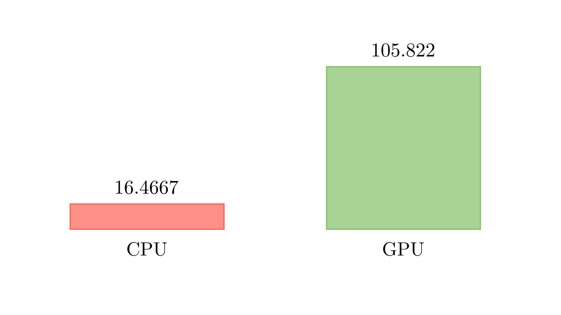
For an image of size \(2048 \times 2048\), it took \(0.0094\) seconds to apply a \(3 \times 3\) filter using my GPU (NVIDIA RTX 3090). This amounts to around \(105\) frames per second (FPS), which is more than sufficient for most image or video-related applications. The table below shows the comparison between the naive CPU and GPU implementation.

Conclusion

Even though 105 FPS is good enough, convolution is an algorithm where I can try other techniques like using constant memory and tiling to reduce global memory accesses. This is the topic for the next blog post.

References

1. Kirk, David B., and W. Hwu Wen-Mei. Programming massively parallel processors: a hands-on approach. Morgan kaufmann, 2016.
2. Ansorge, Richard. Programming in parallel with CUDA: a practical guide. Cambridge University Press, 2022.