YouTube video for this blog
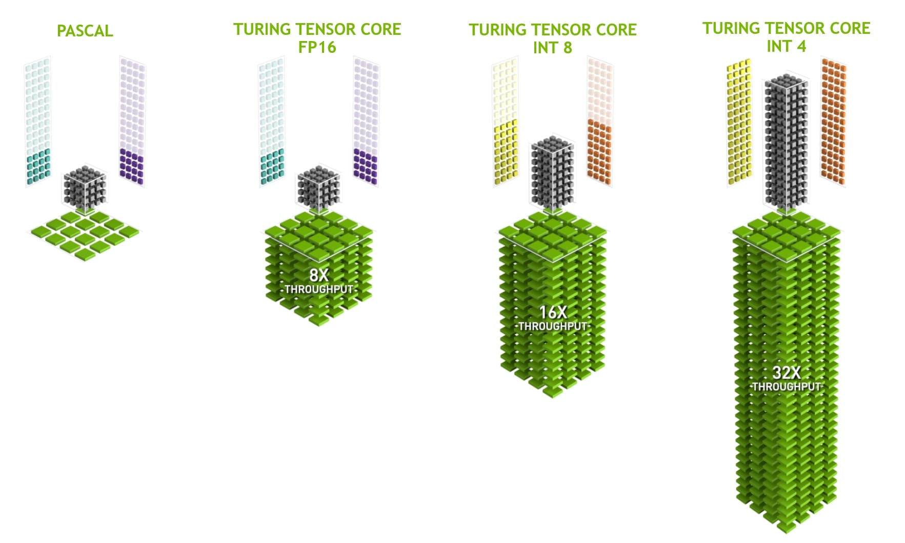
Tensor cores are dedicated accelerator units (somewhat like CUDA cores) on the NVIDIA GPUs (since Volta micro-architecture) that do just one thing: Matrix Multiplication! Dedicated hardware for matrix multiplication makes sense because 90% of the computational cost from AI algorithms is dominated by matrix multiplication, such that over 90% of the computational cost comes from several matrix multiplications. When reading the official NVIDIA documentation, you'll see terms like "half-precision" and "single-precision". I'd like first to understand what this means.
Matrices and Computer Memory
Computer memory is often presented as a linear address space through memory management techniques. This means that we cannot store a matrix in 2D form. Languages like C/C++ and Python store a 2D array of elements in a row-major layout, i.e., in the memory, 1st row is placed after the 0th row, 2nd row after 1st row, and so on.
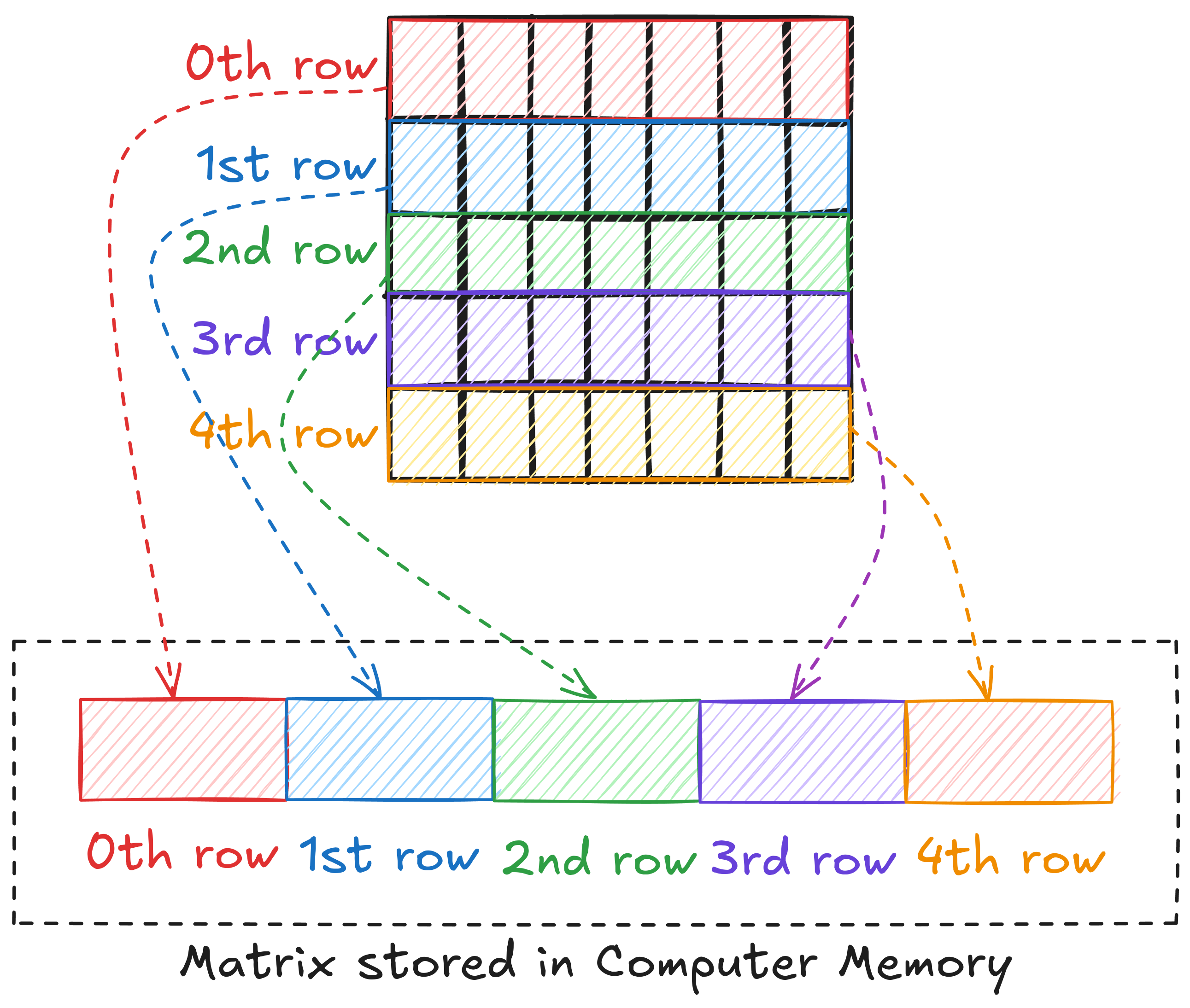
This means that to access an element, we need to linearize the 2D index of the element. For example, if matrix A is M x N, the linearized index of element (6, 8) can be written as 6 x N + 8.
So far, we have discussed matrices in general. Let's now look at what precision means.
Memory Precision
The bit (binary digit) is the smallest and most fundamental digital information and computer memory unit. A byte is composed of 8 bits and is the most common unit of storage and one of the smallest addressable units of memory in most computer architectures. There are several ways to store the numbers in a matrix. The most common one is double precision (declared as double in C/C++). In double precision, a number is stored using 8 consecutive bytes in the memory. Another way is to store the numbers as a single precision type (declared as float in C/C++), where a number is stored using 4 consecutive bytes in the memory. This way, we can store the same number that takes up less space in memory, but we give up accuracy and the range of values we can work with.
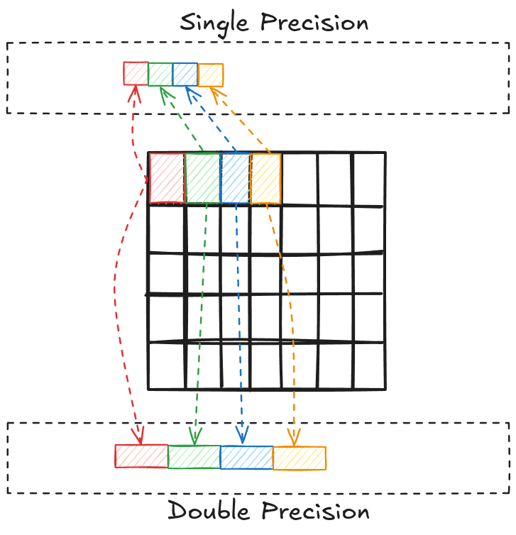
A step further, we have half-precision (2 Bytes) floating point numbers. These are not natively supported in standard C++. However, CUDA has an option to use half-precision (declared as half) and this is where Tensor cores operate.
Tensor Cores Programming
Technically speaking, tensor cores perform matrix multiplication and accumulation, i.e., \(D = A \cdot B + C\). However, we can initialize C to zeros and get matrix multiplication. When working with Tensor cores, the hardware is designed specially so that the input matrices are generally half-precision (FP16) and the output is single-precision (FP32). Tensor cores are restricted to certain matrix dimensions, and Figure 3 shows an example of 4x4 inputs and outputs.

There are other options that you can find in the NVIDIA documentation and moving forward, I will be working with 16x16 matrix dimensions. For an arbitrary matrix size, I must pad the matrices (with zeros) such that they are a multiple of 16 and then perform matrix multiplication using multiple 16x16 tiles. When working with Tensor cores, a big difference (compared to CUDA cores) is that they work on the warp level. This means all threads in a warp (32 threads) cooperate to perform one set of 16x16 matrix multiplication and accumulation.
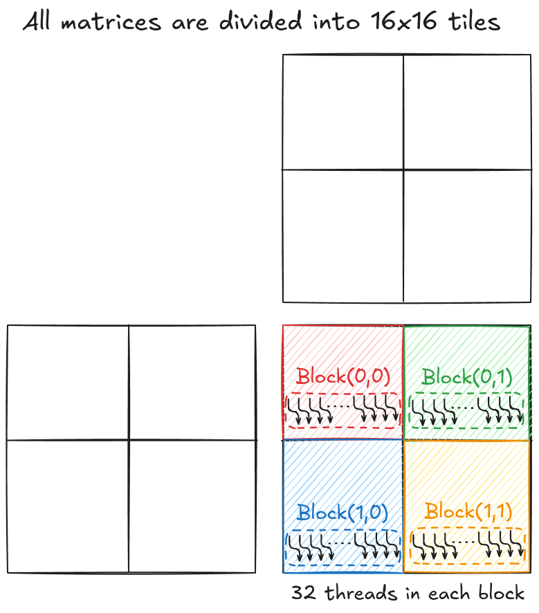
Consider an example where matrices A, B, and C are 32x32. As tensor cores can only work with 16x16 matrices, the idea is to split the 32x32 matrices into 4 tiles (each 16x16). To keep things simple, I will define 4 blocks arranged in a 2x2 grid (shown in Figure 4). Each block has 32 threads (i.e., a single warp) and is responsible for computing 1 tile of the output matrix C.
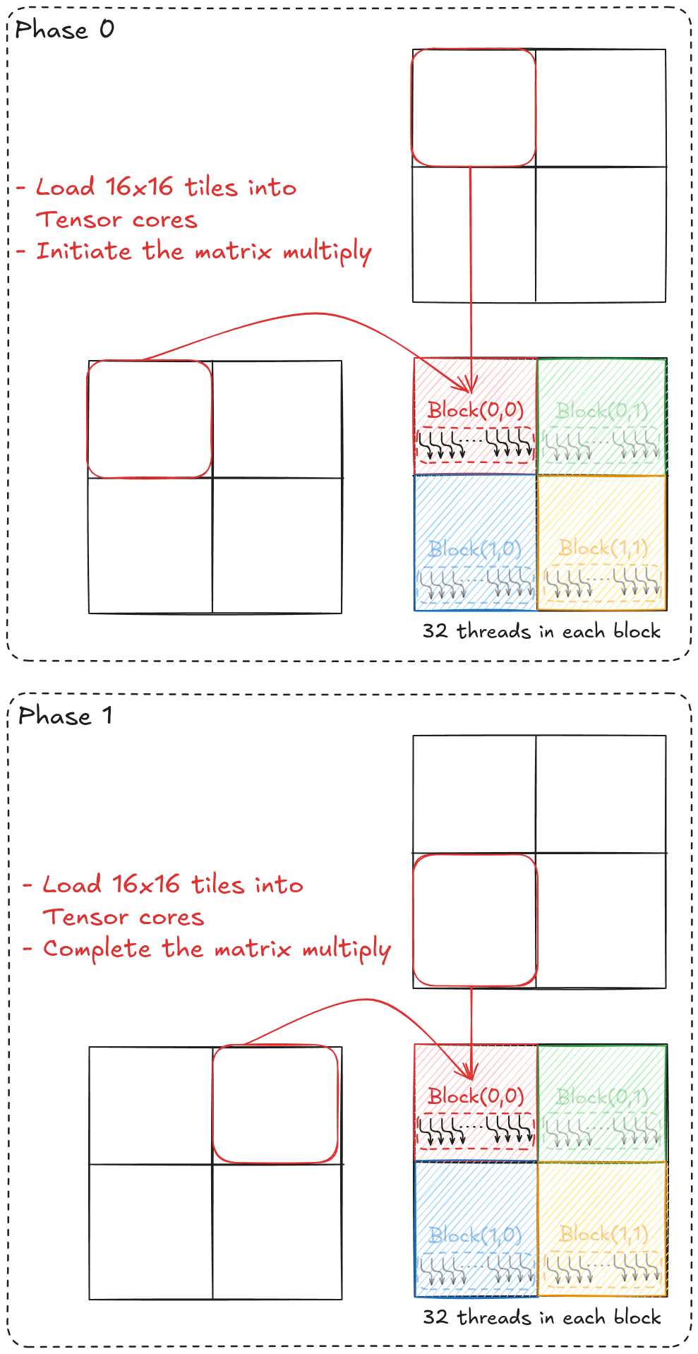
For this example, each tile of D will be computed in two phases. Consider tile(0,0) (shown in Figure 5); in phase 0, all 32 threads cooperatively load tile(0,0) of matrix A and B into tensor cores and perform the partial matrix multiplication. In phase 1, the same 32 threads load tile(0,1) of matrix A and tile(1,0) of matrix B into tensor cores and finish the matrix multiplication.
While coding the general matrix multiplication using tensor cores, the first step is to define the tile sizes. For my GPU, I've set this at 16x16, and then using this alongside the fact that each block has 32 threads, we can define the number of blocks needed.
// WMMA fragment dimensions
const int WMMA_M = 16; // Number rows in tiles of A and C
const int WMMA_N = 16; // Number cols in tiles of B and C
const int WMMA_K = 16; // Number cols in tiles of A or rows in tiles of B

// Kernel execution
dim3 dim_block(32, 1);
dim3 dim_grid(C_n_rows / WMMA_M, C_n_cols / WMMA_N);
Once we have the grid defined, we can start writing the kernel function. Inside the kernel function, we first identify the warp we are working with. Remember that tensor cores work on the warp level, and to keep things simple, I've kept 1 warp per block.
__global__ void naive_tensor_mat_mul_kernel(half *d_A_ptr, half *d_B_ptr, float *d_C_ptr, int C_n_rows, int C_n_cols, int A_n_cols)
{
    // Tile using a 2D grid
    int warpM = blockIdx.x;
    int warpN = blockIdx.y;

    //.
    //.
    //.
}
The next step is to allocate memory for these tiles. Tensor cores work with fragments. Fragments are data structures that represent portions of matrices used in tensor core operations. They are used to load, store, and manipulate matrix data for tensor core computations. On the hardware level, fragments are loaded into registers of warp threads. However, we don't need to worry about moving the data manually. CUDA provides a convenient way to do this, and all we have to do is define the following:
- Whether it's matrix A, B, or C.
- The size of the fragment using
WMMA_M, WMMA_N, WMMA_K. - Precision (half or float) of the data.
- Memory layout (row-major or column-major) of the data.
__global__ void naive_tensor_mat_mul_kernel(half *d_A_ptr, half *d_B_ptr, float *d_C_ptr, int C_n_rows, int C_n_cols, int A_n_cols)
{
    // Tile using a 2D grid
    int warpM = blockIdx.x;
    int warpN = blockIdx.y;

    // Declare the fragments
    nvcuda::wmma::fragment<nvcuda::wmma::matrix_a, WMMA_M, WMMA_N, WMMA_K, half, nvcuda::wmma::row_major> a_frag;
    nvcuda::wmma::fragment<nvcuda::wmma::matrix_b, WMMA_M, WMMA_N, WMMA_K, half, nvcuda::wmma::row_major> b_frag;
    nvcuda::wmma::fragment<nvcuda::wmma::accumulator, WMMA_M, WMMA_N, WMMA_K, float> c_frag;

    //.
    //.
    //.
}We can initialize the output matrix fragment to zeros and split the input matrices into multiple tiles using a loop.
__global__ void naive_tensor_mat_mul_kernel(half *d_A_ptr, half *d_B_ptr, float *d_C_ptr, int C_n_rows, int C_n_cols, int A_n_cols)
{
    // Tile using a 2D grid
    int warpM = blockIdx.x; //(blockIdx.x * blockDim.x + threadIdx.x) / warpSize;
    int warpN = blockIdx.y;

    // Declare the fragments
    nvcuda::wmma::fragment<nvcuda::wmma::matrix_a, WMMA_M, WMMA_N, WMMA_K, half, nvcuda::wmma::row_major> a_frag;
    nvcuda::wmma::fragment<nvcuda::wmma::matrix_b, WMMA_M, WMMA_N, WMMA_K, half, nvcuda::wmma::row_major> b_frag;
    nvcuda::wmma::fragment<nvcuda::wmma::accumulator, WMMA_M, WMMA_N, WMMA_K, float> c_frag;

    // Initialize the output to zero
    nvcuda::wmma::fill_fragment(c_frag, 0.0f);

    // Loop over A_n_cols
    for (int i = 0; i < A_n_cols; i += WMMA_K) {
        //.
        //.
        //.

    }
}
All threads in a warp work together to load the tiles to be computed by tensor cores. All we need to do is point the warp towards the top left element of the tile. We have already defined the size of fragments, so the appropriate tiles will get loaded for the tensor cores using nvcuda::wmma::load_matrix_sync(). Once the tiles are loaded, matrix multiplication using tensor cores is just a single line away using nvcuda::wmma::mma_sync().
__global__ void naive_tensor_mat_mul_kernel(half *d_A_ptr, half *d_B_ptr, float *d_C_ptr, int C_n_rows, int C_n_cols, int A_n_cols)
{
    // Tile using a 2D grid
    int warpM = blockIdx.x; //(blockIdx.x * blockDim.x + threadIdx.x) / warpSize;
    int warpN = blockIdx.y;

    // Declare the fragments
    nvcuda::wmma::fragment<nvcuda::wmma::matrix_a, WMMA_M, WMMA_N, WMMA_K, half, nvcuda::wmma::row_major> a_frag;
    nvcuda::wmma::fragment<nvcuda::wmma::matrix_b, WMMA_M, WMMA_N, WMMA_K, half, nvcuda::wmma::row_major> b_frag;
    nvcuda::wmma::fragment<nvcuda::wmma::accumulator, WMMA_M, WMMA_N, WMMA_K, float> c_frag;

    // Initialize the output to zero
    nvcuda::wmma::fill_fragment(c_frag, 0.0f);

    // Loop over A_n_cols
    for (int i = 0; i < A_n_cols; i += WMMA_K) {
        int aRow = warpM * WMMA_M;
        int aCol = i;
        int bRow = i;
        int bCol = warpN * WMMA_N;

        // Load the inputs
        nvcuda::wmma::load_matrix_sync(a_frag, &d_A_ptr[aRow * A_n_cols + aCol], A_n_cols);
        nvcuda::wmma::load_matrix_sync(b_frag, &d_B_ptr[bRow * C_n_cols + bCol], C_n_cols);

        // Perform the matrix multiplication (c_frag = a_frag*b_frag + c_frag)
        nvcuda::wmma::mma_sync(c_frag, a_frag, b_frag, c_frag);

    }

    //.
    //.
    //.
}
Once we have the final result in the output fragment, it can be put back into the global memory similarly. CUDA provides convenient ways to work with tensor cores, which is a big reason for NVIDIA's success.
__global__ void naive_tensor_mat_mul_kernel(half *d_A_ptr, half *d_B_ptr, float *d_C_ptr, int C_n_rows, int C_n_cols, int A_n_cols)
{
    // Tile using a 2D grid
    int warpM = blockIdx.x; //(blockIdx.x * blockDim.x + threadIdx.x) / warpSize;
    int warpN = blockIdx.y;

    // Declare the fragments
    nvcuda::wmma::fragment<nvcuda::wmma::matrix_a, WMMA_M, WMMA_N, WMMA_K, half, nvcuda::wmma::row_major> a_frag;
    nvcuda::wmma::fragment<nvcuda::wmma::matrix_b, WMMA_M, WMMA_N, WMMA_K, half, nvcuda::wmma::row_major> b_frag;
    nvcuda::wmma::fragment<nvcuda::wmma::accumulator, WMMA_M, WMMA_N, WMMA_K, float> c_frag;

    // Initialize the output to zero
    nvcuda::wmma::fill_fragment(c_frag, 0.0f);

    // Loop over A_n_cols
    for (int i = 0; i < A_n_cols; i += WMMA_K) {
        int aRow = warpM * WMMA_M;
        int aCol = i;
        int bRow = i;
        int bCol = warpN * WMMA_N;

        // Load the inputs
        nvcuda::wmma::load_matrix_sync(a_frag, &d_A_ptr[aRow * A_n_cols + aCol], A_n_cols);
        nvcuda::wmma::load_matrix_sync(b_frag, &d_B_ptr[bRow * C_n_cols + bCol], C_n_cols);

        // Perform the matrix multiplication
        nvcuda::wmma::mma_sync(c_frag, a_frag, b_frag, c_frag);
    }

    // Store the output
    int cRow = warpM * WMMA_M;
    int cCol = warpN * WMMA_N;
    nvcuda::wmma::store_matrix_sync(&d_C_ptr[cRow * C_n_cols + cCol], c_frag, C_n_cols, nvcuda::wmma::mem_row_major);
}
Why GFLOPS?
So far (in the previous blog posts), I've been looking at the execution time. Even though time is a perfectly fine metric to analyze, a better option is to look at the number of operations performed per second by the function or Giga Floating-Point Operations per Second (GFLOPS). When multiplying two M x K and K x N matrices, each output matrix element requires approximately K multiplications and K additions, i.e., 2K operations. As there are total M x N output elements, the total number of operations is 2 x M x N x K. Dividing this number by the time it took to perform matrix multiplication gives FLOPS for the implemented algorithm (that can be converted to GFLOPS).
Benchmark
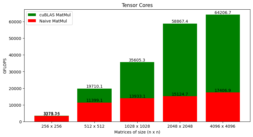
Figure 6 shows the GFLOPS for the tiled version that uses CUDA cores against the naive version that uses tensor cores. The jump in performance is massive (especially for large matrices)!
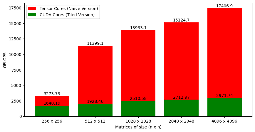
It's not ideal to compare CUDA cores to tensor cores, and the tiled version is not optimal. But so is the version using tensor cores. Figure 7 shows the cuBLAS matrix multiplication against the naive version that I've written.
