Mini Project: GPU Accelerated Image Filters using Convolution
Apply filters to high-resolution images using 2D convolution on a GPU. Along the way, learn about caches and using constant, shared, and pinned memory.

YouTube video

Code repository
A while ago, I was going through the pics from my last vacation, casually editing using the built-in filters in the Photos app, and I never really paid attention before that the whole process is quite snappy. This led me to think about whether I could build something similar. Apple or Google conducts extensive research in image processing; I cannot match that. Image processing is not my expertise, and I want to keep things simple. Then I remembered a neat little algorithm (from my undergrad days) called convolution.
This mini-project is all about applying filters to high-resolution images using convolution and accelerating the whole process using a GPU. I will show how you can apply five different filters (see Figure 0.1) using a single algorithm and, at the same time, improve the application runtime by \(11\text{x}\) using a GPU (compared to a basic CPU implementation).

Convolution
Convolution is an array operation in which each output element is a weighted sum of the corresponding input elements and a collection of several neighboring elements (symmetric around the location being computed). The weights used in the calculations are defined by a filter array known as a convolution filter or simply filter. The size of the filter is an odd number \((2r+1)\), such that the weighted sum calculation is symmetric around the element being calculated. Convolutions can be 1D, 2D or 3D.
Consider an example involving 1D convolution where the input array is of length \(5\) and filter of size \(3\) (i.e., radius \(1\)). Figure 0.2 shows how the convolution is applied in this case. An important thing to note is how the 1st and last element is computed. Boundary conditions naturally arise here, and the missing input elements (there is just one in this case) are set to \(0\). These missing input elements are referred to as ghost cells.
Figure 0.2: 1D convolution using a filter of radius \(1\).
2D convolution works exactly the same, but the input array and filter are both 2D. Figure 0.3 shows 2D convolution on a \(5 \times 5\) input image using \(3 \times 3\) filter.
Figure 0.3: 2D convolution using a filter of radius \(1 \times 1\).
CPU Implementation
Sequential implementation using a CPU is pretty straightforward. The function cpu_conv2d accepts input image N, filter matrix F, output image P, filter radius r, and the input/output image dimensions (n_rows and n_cols).
/*
Input Image: N
Filter: F
Output Image: P
Filter Radius: r
Num of rows in input/output image: n_rows
Num of cols in input/output image: n_cols
*/
void cpu_conv2d(float *N, float *F, float *P, int r, int n_rows, int n_cols)
{

}
The strategy to perform 2D convolution can be summed up as follows (with the complete code shown in Figure 0.4):
- Loop over each output element. For each output element:
- Loop over the elements of the filter matrix.
- Figure out filter to input element mapping.
- Check for ghost cells and perform the calculations involving input and filter elements.
/*
Input Image: N
Filter: F
Output Image: P
Filter Radius: r
Num of rows in input/output image: n_rows
Num of cols in input/output image: n_cols
*/
void cpu_conv2d(float *N, float *F, float *P, int r, int n_rows, int n_cols)
{
    // 1. Loop over elements of output matrix P
    for (int out_col = 0; out_col < n_rows; out_col++)
    {
        for (int out_row = 0; out_row < n_cols; out_row++)
        {
            // Output in the register
            float p_val = 0.0f;

            // 1a. Loop over elements of the filter F
            for (int f_row = 0; f_row < 2*r+1; f_row++)
            {
                for (int f_col = 0; f_col < 2*r+1; f_col++)
                {
                    // 1b. Input-filter mapping
                    int in_row = out_row + (f_row - r);
                    int in_col = out_col + (f_col - r);

                    // 1c. Ignore computations involving ghost cells
                    if ((in_row >= 0 && in_row < n_rows) && (in_col >= 0 && in_col < n_cols))
                        p_val += F[f_row*(2*r+1) + f_col] * N[in_row*n_cols + in_col];
                }
            }
            // Update value in the output matrix
            P[out_row*n_cols + out_col] = p_val;
        }
    }
}
Figure 0.4: 2D convolution on a CPU.
Benchmarking
For an image of size \(2048 \times 2048\), it took \(0.060\) seconds to apply a \(3 \times 3\) filter using my CPU (AMD Ryzen™ 7 7700). While this is not too bad, it amounts to around \(16\) frames per second (FPS). On a live video feed, where \(24\) FPS (or even \(60\) FPS) is normal, this might not be good enough.
What next?
This three-part blog post series discusses accelerating convolution using a GPU and achieving over \(100\) FPS performance. Specifically, I will be discussing:
- Naive GPU implementation using CUDA C++.
- Using constant memory to store filter matrix and tiling to reduce global memory accesses.
- Using pinned global memory to speed up data transfer between CPU and GPU memory.
Chapter 1: Parallel Convolution on a GPU
Looking at the convolution algorithm, it's easy to see that it can be parallelized effectively, as each output element can be computed independently. The most basic implementation would involve assigning each thread to compute one output element. Considering 2D convolution on a \(5 \times 5\) input image (which gives an output image of the same size), I decided to use \(3 \times 3\) blocks and \(2 \times 2\) grid such that the GPU threads span all the output elements (see Figure 1.1).
Figure 1.1: Parallel 2D convolution using GPU threads.
GPU Implementation
Once the data has been moved to the GPU memory, I can define the thread organization in two lines of code.
// Defining 16 x 16 block
dim3 dim_block(16, 16, 1);

// Defining grid to cover all output elements
dim3 dim_grid(ceil(n_cols/(float)(16)), ceil(n_rows/(float)(16)), 1);
Remember that each thread executes the same kernel function. I first need to get the thread to output element mapping. Kernel function definition is very similar to the cpu_conv2d() function defined in the previous blog post. The main difference is that the input pointers point to the GPU memory locations.
__global__ void gpu_conv2d_kernel(float const *d_N_ptr, float const *d_F_ptr, float *d_P_ptr, int const n_rows, int const n_cols)
{
    // Which output element this thread works on (Thread to output element mapping)
    int const out_col = blockIdx.x*blockDim.x + threadIdx.x;
    int const out_row = blockIdx.y*blockDim.y + threadIdx.y;
}
The strategy for the rest of the kernel function can be summed up as follows (with the complete code shown in Figure 1.2):
- Some threads map to the elements outside the matrix's bounds, i.e., invalid locations (see Figure 1.2). I must turn these threads off so they don't corrupt the final results.
Figure 1.2: Thread to element mapping with invalid threads highlighted.
- Each thread loops over the elements of the filter matrix (see Figure 1.3).
- Figures out filter to input element mapping.
- Check for ghost cells (in the input matrix) and perform input and filter elements calculations.
Figure 1.3: Each thread loops over the filter elements one by one (and checks for ghost cells along the way).
- Each thread stores the final result back in the output matrix.
__global__ void gpu_conv2d_kernel(float const *d_N_ptr, float const *d_F_ptr, float *d_P_ptr, int const n_rows, int const n_cols)
{
    // Which output element this thread works on (Thread to output element mapping)
    int const out_col = blockIdx.x*blockDim.x + threadIdx.x;
    int const out_row = blockIdx.y*blockDim.y + threadIdx.y;

    // 1. Check if output element is valid
    if (out_row < n_rows && out_col < n_cols)
    {
        // Result (in thread register)
        float p_val = 0.0f;

        // 2. Loop over elements of the filter array (FILTER_RADIUS is defined as a constant)
        #pragma unroll
        for (int f_row = 0; f_row < 2*FILTER_RADIUS+1; f_row++)
        {
            for (int f_col = 0; f_col < 2*FILTER_RADIUS+1; f_col++)
            {
                // 2a. Input element to filter element mapping
                int in_row = out_row + (f_row - FILTER_RADIUS);
                int in_col = out_col + (f_col - FILTER_RADIUS);

                // 2b. Boundary check (for ghost cells)
                if (in_row >= 0 && in_row < n_rows && in_col >= 0 && in_col < n_cols)
                    p_val += d_F_ptr[f_row*(2*FILTER_RADIUS+1) + f_col] * d_N_ptr[in_row*n_cols + in_col]; // Computations
            }
        }
        // 3. Storing the final result in output matrix
        d_P_ptr[out_row*n_cols + out_col] = p_val;
    }
}
Figure 1.4: 2D convolution on a GPU with boundary condition handling.
Benchmarking
For an image of size \(2048 \times 2048\), it took \(0.0094\) seconds to apply a \(3 \times 3\) filter using my GPU (NVIDIA RTX 3090). This amounts to around \(105\) frames per second (FPS), which is more than sufficient for most image or video-related applications. The table below shows the comparison between the naive CPU and GPU implementation.
| CPU | GPU (Naive) | |
|---|---|---|
| Total execution time (seconds) | 0.0607285 | 0.00931497 |
Even though 105 FPS is good enough, convolution is an algorithm where I can try other techniques like using constant memory and tiling to reduce global memory accesses.
Chapter 2: Using Constant Memory and Tiling to reduce Global Memory Accesses
The kernel function from Chapter 1 (shown in Figure 2.1) has a big problem (at least theoretically). It is accessing all of the required data from global memory! I've discussed (in a previous blog post) that accessing data straight from global memory is not ideal as it has long latency and low bandwidth. A common strategy is to move a subset of the data to faster (but much smaller) memory units and then repeatedly access these memory units that provide faster access and high bandwidth.
__global__ void gpu_conv2d_kernel(float const *d_N_ptr, float const *d_F_ptr, float *d_P_ptr, int const n_rows, int const n_cols)
{
    // Which output element this thread works on (Thread to output element mapping)
    int const out_col = blockIdx.x*blockDim.x + threadIdx.x;
    int const out_row = blockIdx.y*blockDim.y + threadIdx.y;

    // 1. Check if output element is valid
    if (out_row < n_rows && out_col < n_cols)
    {
        // Result (in thread register)
        float p_val = 0.0f;

        // 2. Loop over elements of the filter array (FILTER_RADIUS is defined as a constant)
        #pragma unroll
        for (int f_row = 0; f_row < 2*FILTER_RADIUS+1; f_row++)
        {
            for (int f_col = 0; f_col < 2*FILTER_RADIUS+1; f_col++)
            {
                // 2a. Input element to filter element mapping
                int in_row = out_row + (f_row - FILTER_RADIUS);
                int in_col = out_col + (f_col - FILTER_RADIUS);

                // 2b. Boundary check (for ghost cells)
                if (in_row >= 0 && in_row < n_rows && in_col >= 0 && in_col < n_cols)
                    p_val += d_F_ptr[f_row*(2*FILTER_RADIUS+1) + f_col] * d_N_ptr[in_row*n_cols + in_col]; // Computations
            }
        }
        // 3. Storing the final result in output matrix
        d_P_ptr[out_row*n_cols + out_col] = p_val;
    }
}
Figure 2.1: 2D convolution on a GPU with boundary condition handling.
GPU Memory Units
I've previously discussed GPU memory hierarchy in detail. However, I did not cover specialized memory units like constant memory and texture memory. In this section, I will put everything together and discuss different memory units in a GPU from a programmer's point of view.
GPU is organized as an array of SMs, but programmers never interact with SMs directly. Instead, they use programming constructs like thread and thread blocks to interface with the hardware. GPU memory is divided into two parts (see Figure 2.2): off-chip and on-chip memory.
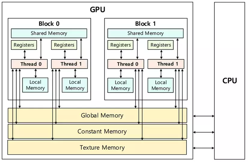
Off-chip Memory Units
- Global memory is the largest off-chip memory unit (a few GBs).
- It has long latency and low bandwidth but can be accessed by all the threads in a grid.
- Global memory in CUDA devices is implemented using DRAM (Dynamic Random Access Memory) technology, which is quite slow compared to modern computing devices.
- As the DRAM access speed is relatively slow, parallelism is used to increase the rate of data access (also known as memory access throughput).
- This parallelism requires optimization from a programmer and is contingent on coalesced memory access. For more information, check out the section in a previous blog post: How to improve Kernel Performance?
- Constant memory is a much smaller off-chip memory unit (~64 KB) that can be used for constant values.
- Constant memory is optimized for broadcast, where all threads in a warp read the same memory location.
- It is a faster memory unit than the global memory and can be accessed by all threads in a grid. However, the threads can't modify the contents during kernel execution (it's a read-only memory unit).
- For read-only memory units like constant memory, the hardware can be designed specifically in a highly efficient manner.
- Supporting high-throughput writes into a memory unit requires sophisticated hardware logic. As constant memory variables are constant during the kernel execution, it does not require writes, hence the manufacturer can do away with the sophisticated logic which will reduce the price and the power consumption of the overall hardware.
- Furthermore, constant memory is around 64 KB in size, which requires a smaller area (physically) on the board. This will, in turn, further reduce the power consumption and the price.
- Texture memory is another specialized off-chip memory unit optimized for textures.
- All threads in a grid can access it.
- Texture memory somewhat lies in between the global and constant memory:
- It is smaller than global memory but larger than constant memory.
- Data accesses from texture memory are faster than global memory but slower than constant memory.
- Texture memory is optimized for 2D spatial locality, making it ideal for 2D and 3D data structures.
On-chip Memory Units
On-chip memory units reside near the cores. Hence, data access from on-chip memory is blazing fast. The issue in this case is that the size of these memory units is extremely small (maximum of ~16KB per SM). There are three main types of on-chip memory units:
- Shared Memory
- Shared memory is a small memory space (~16KB per SM) that resides on-chip and has a short latency with high bandwidth.
- On a software level, it can only be written and read by the threads within a block.
- Registers
- Registers are extremely small (~8KB per SM) and extremely fast memory units that reside on-chip.
- On a software level, it can be written and read by an individual thread (i.e., private to each thread).
- Local Memory
- It is local to each thread and is (mostly) used to store temporary variables.
- It has the smallest scope and is dedicated to each individual thread.
Constant Memory
Figure 2.1 shows that I'm accessing the filter matrix and the input image matrix from the global memory. One thing to keep in mind is that input images are high resolution (i.e., \(\approx 2000 \times 2000 \)), while the filter matrix is much much smaller (mostly \( 3 \times 3\) or \( 5 \times 5\) or \( 7 \times 7\)). I can use constant memory for the filter array because:
- It is small in size and can easily fit in the constant memory.
- It does not change during the execution of the kernel, i.e., I only need to read the values.
- All threads access the filter elements in the same order (starting from
F[0][0]and moving by one element at a time), and constant memory is optimized for such accesses.
To use constant memory, the host cost must allocate and copy constant memory variables in a way different than the global memory variables.
// Compile-time constant
#define FILTER_RADIUS 2

// Allocate constant memory
__constant__ float F[2*FILTER_RADIUS+1][2*FILTER_RADIUS+1];

// Move data from host memory to constant memory (Destination, Source, Size)
cudaMemcpyToSymbol(F, F_h, (2*FILTER_RADIUS+1)*(2*FILTER_RADIUS+1)*sizeof(float));F_h on the host memory.Kernel function accesses constant memory variables like global variables, i.e., I do not need to pass them as arguments to the kernel. Figure 2.3 shows the revised version that assumes a filter d_F in the constant memory.
#define FILTER_RADIUS 1
extern __constant__ float d_F[(2*FILTER_RADIUS+1)*(2*FILTER_RADIUS+1)];

__global__ void gpu_conv2d_constMem_kernel(float const *d_N_ptr, float *d_P_ptr, int const n_rows, int const n_cols)
{
    // Which output element does this thread work on
    int const out_col = blockIdx.x*blockDim.x + threadIdx.x;
    int const out_row = blockIdx.y*blockDim.y + threadIdx.y;

    // Check if output element is valid
    if (out_row < n_rows && out_col < n_cols)
    {
        // Result (in thread register)
        float p_val = 0.0f;

        // Loop over elements of the filter array
        #pragma unroll
        for (int f_row = 0; f_row < 2*FILTER_RADIUS+1; f_row++)
        {
            for (int f_col = 0; f_col < 2*FILTER_RADIUS+1; f_col++)
            {
                // Input element to filter element mapping
                int in_row = out_row + (f_row - FILTER_RADIUS);
                int in_col = out_col + (f_col - FILTER_RADIUS);

                // Boundary Check
                if (in_row >= 0 && in_row < n_rows && in_col >= 0 && in_col < n_cols)
                    p_val += d_F[f_row*(2*FILTER_RADIUS+1) + f_col] * d_N_ptr[in_row*n_cols + in_col];
            }
        }
        d_P_ptr[out_row*n_cols + out_col] = p_val;
    }
}
Figure 2.3: 2D convolution kernel using constant memory with boundary condition handling.
d_F is visible to the kernel. In short, all C language scoping rules for global variables apply here!Tiled Convolution using Shared Memory
Now that the filter matrix is handled let's focus on reducing global memory access for the input image. The strategy here is to partition the output image into multiple tiles (output tiles) and assign each to a unique block. Figure 2.4 shows that a larger input tile (blue) is required to compute an output tile (green). This complicates things, but one way to solve this problem is by keeping the block dimension equal to the input tile dimension. This will result in a simpler data transfer from global to shared memory, but the final computation of the output tile will be complicated.
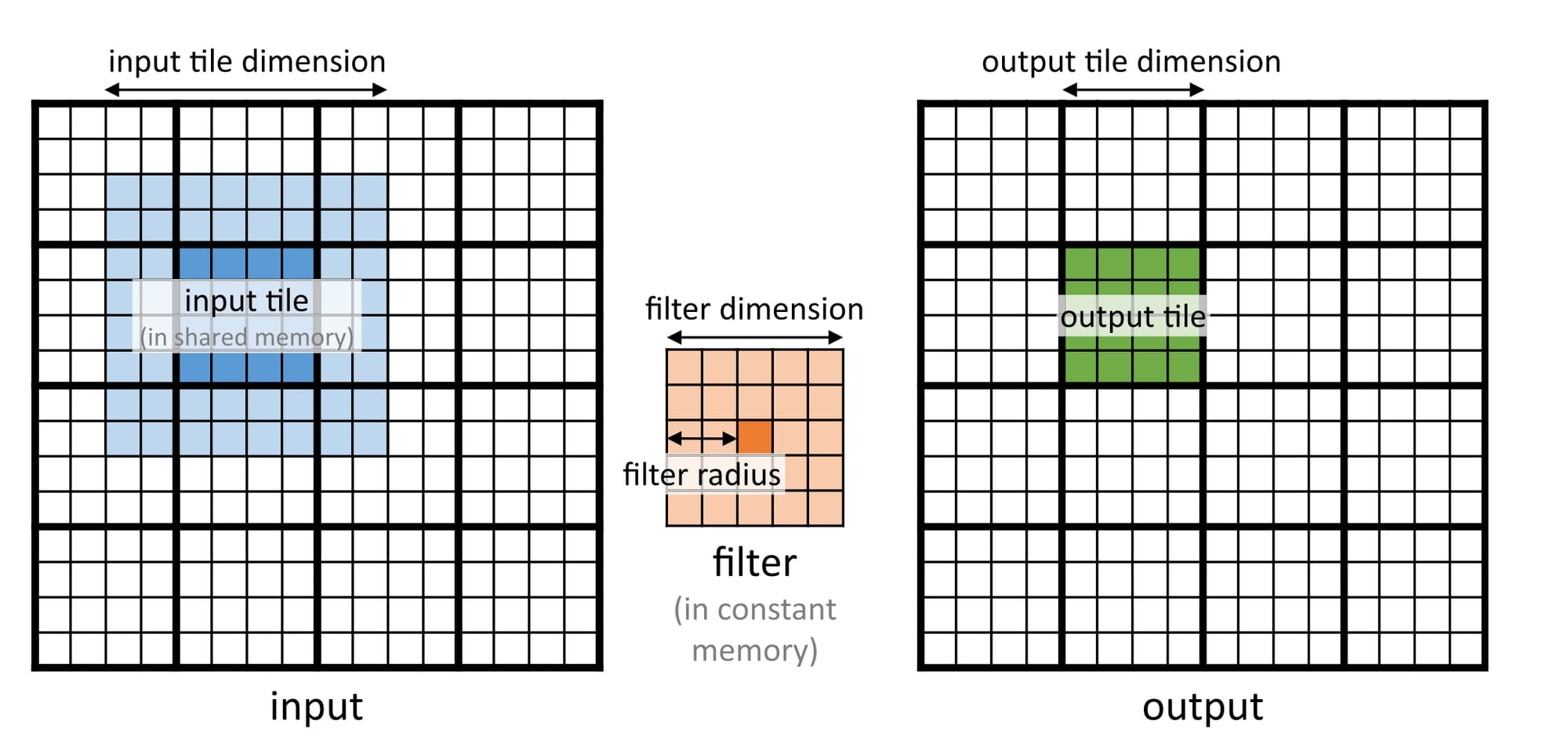
Consider an example where the input and output are \(16 \times 16\) and the filter is \(5 \times 5\). I use a block to compute a \(4 \times 4\) output tile. Remember that to compute this \(4 \times 4\) output tile, I will need an \(8 \times 8\) input tile. So, the block dimension will be \(8 \times 8\) with a \(4 \times 4\) grid (to cover all the output elements). Figure 2.5 shows the thread-to-element mapping for both input and output tiles. Notice how it naturally aligns with the input tile elements, but some of the threads lie outside the range for the output tile. I must disable these while computing the final answer.
Figure 2.5: Applying tiling to 2D convolution.
I can write the kernel function in __ steps:
- The kernel function starts with mapping the threads to output elements. Remember that the thread block is shifted relative to the output tile (Figure 2.5).
- Next, shared memory is allocated.
- Once allocated, the input tile is copied into this shared memory. Copying the data is pretty straightforward, except I need to check for ghost cells (see Figure 2.6).
- Barrier synchronization must be used to ensure that the complete input tile has been loaded.
Figure 2.6: Loading input tile into shared memory
- Once the shared memory is populated, I can proceed to the computations.
- The first check ensures that threads lie within the output image bounds (output ghost elements).
- The second check ensures that the threads lie within the output tile bounds.
- After all the checks, the code loops over the filter elements.
- Inside this loop, the mapping to the elements in the shared memory is defined, and computations are performed.
- Finally, the results are stored back in the output array.
Figure 2.7 shows the complete code.
#define FILTER_RADIUS 1
#define INPUT_TILE_DIM 16
#define OUTPUT_TILE_DIM (INPUT_TILE_DIM - 2*FILTER_RADIUS)

extern __constant__ float d_F[(2*FILTER_RADIUS+1)*(2*FILTER_RADIUS+1)];

__global__ void gpu_conv2d_tiled_kernel(float *d_N_ptr, float *d_P_ptr, int n_rows, int n_cols)
{
    // 1. Which output element does this thread works on
    int out_col = blockIdx.x*OUTPUT_TILE_DIM + threadIdx.x - FILTER_RADIUS;
    int out_row = blockIdx.y*OUTPUT_TILE_DIM + threadIdx.y - FILTER_RADIUS;

    // 2. Allocate shared memory
    __shared__ float N_sh[INPUT_TILE_DIM][INPUT_TILE_DIM];

    // 2a. Checking for ghost cells and loading tiles into shared memory
    if (out_row >= 0 && out_row < n_rows && out_col >= 0 && out_col < n_cols)
        N_sh[threadIdx.y][threadIdx.x] = d_N_ptr[out_row*n_cols + out_col];
    else
        N_sh[threadIdx.y][threadIdx.x] = 0.0f;

    // 2b. Ensure all elements are loaded
    __syncthreads();

    // 3. Computing output elements
    int tile_col = threadIdx.x - FILTER_RADIUS;
    int tile_row = threadIdx.y - FILTER_RADIUS;

    // 3a. Check if the output element is valid
    if (out_row >= 0 && out_row < n_rows && out_col >= 0 && out_col < n_cols)
    {
        // 3b. Checking for threads outside the tile bounds
        if (tile_row >= 0 && tile_row < OUTPUT_TILE_DIM && tile_col >= 0 && tile_col < OUTPUT_TILE_DIM)
        {
            // Result (in thread register)
            float p_val = 0.0f;

            // 3c. Loop over elements of the filter array
            #pragma unroll
            for (int f_row = 0; f_row < 2*FILTER_RADIUS+1; f_row++)
            {
                for (int f_col = 0; f_col < 2*FILTER_RADIUS+1; f_col++)
                {
                    // 3d. Input element (in shared memory) to filter element mapping
                    int in_row = tile_row + f_row;
                    int in_col = tile_col + f_col;

                    p_val += d_F[f_row*(2*FILTER_RADIUS+1) + f_col] * N_sh[in_row][in_col];
                }
            }

            // 4. Storing the final result
            d_P_ptr[out_row*n_cols + out_col] = p_val;
        }
    }
}
Figure 2.7: Tiled 2D convolution using shared memory.
Benchmarking
The table below compares application runtime for different versions of 2D convolution for an image of size \(2048 \times 2048\) and a \(3 \times 3\) filter:
| CPU (Naive) | GPU (Naive) | GPU (Constant Memory only) | GPU (Constant Memory + Tiling) | |
|---|---|---|---|---|
| Total execution time (seconds) | 0.0607 | 0.00944 | 0.00916 | 0.00939 |
This is unexpected. There is almost no improvement when using constant memory or tiling!
Using constant and shared memory (via tiling) are two important concepts in GPU programming (even though it didn't improve things practically). However, I don't want to leave this without any analysis. Next, I will analyze why I couldn't improve the performance using constant and shared memory and if there is anything else that I can do to reduce the application runtime.
Chapter 3: GPU Caches and Pinned Memory
So far, I have not gotten any meaningful improvement over the naive GPU implementation of 2D convolution (the table below shows runtime). I will first start with a detailed runtime analysis and try to see the bottlenecks.
| GPU (Naive) | GPU (Constant Memory only) | GPU (Constant Memory + Tiling) | |
|---|---|---|---|
| Total execution time (seconds) | 0.00944 | 0.00916 | 0.00939 |
Running any application on a GPU involves four broad steps:
- Allocating GPU memory
- Transferring data from CPU (RAM) to GPU global memory (VRAM).
- Performing calculations using the GPU cores.
- Transferring results from GPU global memory (VRAM) to CPU memory (RAM).
The table below shows the detailed breakdown of the runtimes.
| GPU (Naive) | GPU (Constant Memory only) | GPU (Constant Memory + Tiling) | |
|---|---|---|---|
| Memory Allocation time (seconds) | 0.000108 | 0.000262 | 0.000228 |
| CPU to GPU Transfer time (seconds) | 0.00327 | 0.00302 | 0.00298 |
| Kernel execution time (seconds) | 4.606e-05 | 5.824e-05 | 5.750e-05 |
| GPU to CPU Transfer time (seconds) | 0.00602 | 0.00582 | 0.00611 |
| Total execution time (seconds) | 0.00944 | 0.00916 | 0.00939 |
It is clear that data transfer to and from GPU is the major bottleneck! It is around two orders of magnitude slower than the kernel execution, and if I have to decrease the overall runtime, I must reduce the data transfer speeds. There is an easy way to do that, but I want to first understand why isn't kernel runtime improvement with the use of constant memory and shared memory?
Caches
Figure 3.1 shows the physical view of the GPU hardware. The GPU is organized into an array of highly threaded streaming multiprocessors (SMs). Each SM has several processing units called streaming processors or CUDA cores (shown as green tiles inside SMs) that share control logic. The SMs also contain a different on-chip memory shared amongst the CUDA cores inside the SM (known as shared memory). GPU also has a much larger (and slower) off-chip memory, the main component of which is the global memory or VRAM.
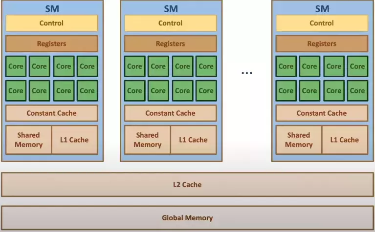
Modern processors employ cache memories to mitigate the effect of long latency and low bandwidth of global memory. Unlike the CUDA shared memory, caches are transparent to programs. This means the program accesses the global memory variables, but the hardware automatically retains the most recent or frequently used cache variables. Whenever the same variable is accessed later, it will be served from the cache, eliminating the need to access VRAM.
Due to the trade-off between the size and the memory speed, modern processors often employ multiple levels of caches (as shown in Figure 3.1). L1 cache runs at a speed close to that of the processor (but very small in size). The L2 cache is relatively large but takes tens of cycles to access. They are typically shared among multiple processor cores or SMs in a CUDA device, so the access bandwidth is shared among SMs.
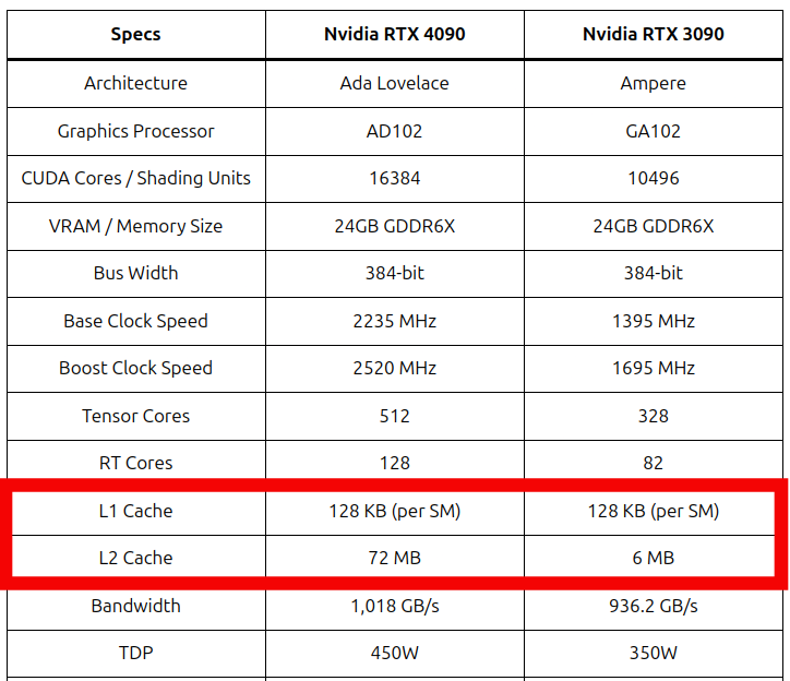
Looking at my 2D convolution code, there are two things that stand out:
- The input image is relatively small (\(2048 \times 2048\) pixels), and the filter is even smaller (\(3 \times 3\)): Modern NVIDIA GPUs have large enough caches (see Figure 3.2) to fit a large chunk of the data, such that global memory accesses are reduced automatically.
- To compute one output element, I'm performing 9 multiplications and 9 additions: There is an overhead related to the data transfer when using constant or shared memory. The idea behind using these memory units is that much faster calculations can compensate the performance loss, and as there aren't that many calculations to perform, there is no significant improvement.
With this out of the way, I can finally move on to reducing the CPU to GPU (and vice-versa) data transfer times.
Pinned Memory
Modern computing systems can be viewed from a physical or logical perspective. Just like GPUs, where on the physical level, we have SMs, CUDA cores, caches, etc. Programmers rarely even interact with hardware directly. Instead, they use logical constructs like threads, blocks, and grids to interface with the hardware.
Similarly, with the CPU memory (RAM), there are two perspectives:
- Physical Memory: This represents the memory cells installed on the motherboard like RAM.
- Virtual Memory: This abstract concept makes it easy for the programmer to manage memory. The operating system creates it, and the CPU maps the logical memory to the physical address in RAM.
By default, CPU-allocated memory is paced physically in RAM and logically in pageable memory. The issue with pageable memory is that the data can be swapped automatically between RAM and slower memory units like HDD (to keep RAM free for other processes). This means that when I try to transfer the data from the CPU to the GPU, it might not be readily available on the RAM! To mitigate this, I can use pinned memory. Data in the pinned memory cannot be moved away from the RAM and will 100% be there whenever data transfer is required.
Using pinned memory is very easy. CUDA provides an API function cudaMallocHost() that allocates the pinned memory. I only have to use this function to allocate the host memory, and the rest of the program stays exactly the same. Figure 3.3 shows an example where I use pinned memory for input and output images.
int main(int argc, char const *argv[])
{
    // Allocate pinned memory for the images (input and output)
    float* N;
    err = cudaMallocHost((void**)&N, 2048*2048*sizeof(float));
    cuda_check(err);

    float *P;
    err = cudaMallocHost((void**)&P, 2048*2048*sizeof(float));
    cuda_check(err);

    // .
    // .
    // .
}
Figure 3.3: Using pinned memory.
Benchmarking
The table below shows the detailed benchmarks for the naive GPU implementation using pageable and pinned memory.
| GPU (Naive) using Pageable Memory | GPU (Naive) using Pinned Memory | |
|---|---|---|
| Memory Allocation time (seconds) | 0.000108 | 0.000217 |
| CPU to GPU Transfer time (seconds) | 0.00327 | 0.00265 |
| Kernel execution time (seconds) | 4.606e-05 | 4.507e-05 |
| GPU to CPU Transfer time (seconds) | 0.00602 | 0.00249 |
| Total execution time (seconds) | 0.00944 | 0.00542 |
Using pinned memory, the runtime is almost halved! This is a decent uplift because the application runs at around 184 FPS compared to 105 FPS when pageable memory was used.
Application Demo
For the final application, I decided to use pinned memory on the CPU side and constant memory on the GPU side. I'm not using shared memory via tiling as I don't want to complicate my codebase for negligible performance uplift (if that).
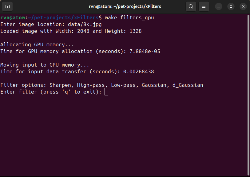
I've used Makefile to make compilation (and execution) easy. All I have to do is run a simple command make filters_gpu, and it will automatically compile the source code and run the executable. This will prompt an input from the user to type in the filter of choice (see Figure 3.4).
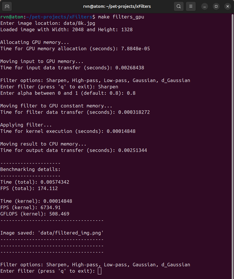
Let's say I decided to use the Sharpen filter. In this case, it will ask me to enter the sharpen strength (between 0 and 1), and I decided to use 0.8. After this, the program will apply the filter to the supplied image and store back the output image on the disk. The terminal will display all the information, including detailed benchmarks (see Figure 3.5). Figure 3.6 shows the original image alongside the filtered image.

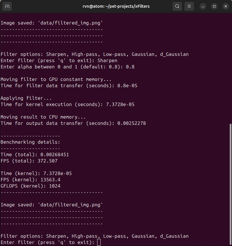
I've written this code considering the user can try multiple filters on the same image. I want the application to reuse the image already in the GPU global memory (as that is a bottleneck), which results in the 2nd run being much faster. Figure 3.6 shows that the total FPS now is over 372 (compared to 174 in Figure 3.5).
Conclusion
I explored several topics in this mini-project, and the summary is as follows:
- 2D convolution can be accelerated significantly using a GPU.
- When the application is computationally light (relatively), using specialized memory units like constant or shared memory might not significantly improve.
- using pinned memory can significantly accelerate the data transfer between CPU and GPU memory.
References
- YouTube video
- Code repository

- Programming Massively Parallel Processors: A Hands-on Approach
Kirk, David B., and W. Hwu Wen-Mei. Programming massively parallel processors: a hands-on approach. Morgan kaufmann, 2016.
- Programming in parallel with CUDA: a practical guide
Ansorge, Richard. Programming in parallel with CUDA: a practical guide. Cambridge University Press, 2022.
- Memory types in GPU by CisMine Ng

- Pinned Memory by CisMine Ng

- Stack Overflow: Shouldn't be 3x3 convolution much faster on GPU (OpenCL)