By Tushar Gautam in GPGPU Programming — 28 Nov 2024

Mini Project: GPU Accelerated Matrix Multiplication (almost) like cuBLAS

Learn CUDA C/C++ basics by working on a single application: matrix multiplication. To make things interesting, let us try to match the performance of NVIDIA cuBLAS.

Photo by Caspar Camille Rubin / Unsplash

YouTube video

I will show you two plots side by side. Figure 0.1 shows the Google Trends graph for interest in AI, and Figure 0.2 shows the stock chart on NVIDIA's website.

Figure 0.1: Google Trends showing the interest in AI

Figure 0.2: NVIDIA Stock Chart (as of September 2024)

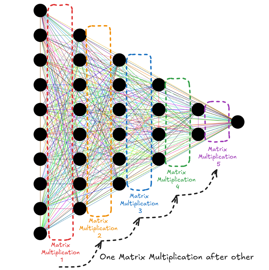
It is no coincidence that as the interest in AI rose, so did the NVIDIA stock value. In the last 10 years or so, the field of AI has been dominated by algorithms using neural networks at their heart. And, at the heart of neural nets, there's matrix multiplication. Over 90% of the neural net's compute cost comes from several matrix multiplications done one after the other [1].

Figure 0.3: Neural nets are (kind of!) nothing but a series of matrix multiplications

But why does NVIDIA benefit from this? Anyone can do matrix multiplication. I can write it myself in under 15 lines of C++ code.

void matrix_multiplication(float *A_mat, float *B_mat, float *C_mat, int n)
{
    for (int row = 0; row < n; row++)
    {
        for (int col = 0; col < n; col++)
        {
            float val = 0.0f;
            for (int k = 0; k < n; k++)
            {
                val += A_mat[row*n + k] * B_mat[k*n + col];
            }
            C_mat[row*n + col] = val;
        }
    }
}

Matrix Multiplication involving square matrices of size n x n

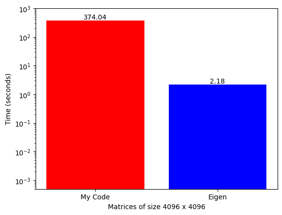
Even better, I can use an open-source library like Eigen.

#include <Eigen/Dense>

int main(int argc, char const *argv[])
{
    // .
    // .
    // .
    
    // Generate Eigen square matrices A, B and C
    // .
    // .
    // .
    
    // Perform matrix multiplication: C = A * B 
    C_eigen = A_eigen * B_eigen;

    // .
    // .
    // .

    return 0;
}

Matrix Multiplication using Eigen

However, when performing matrix multiplication on large matrices, which is common in modern neural networks, the computational time becomes prohibitively long. The duration of a single matrix multiplication operation can be so extensive that it becomes impractical to build large neural networks using these libraries.

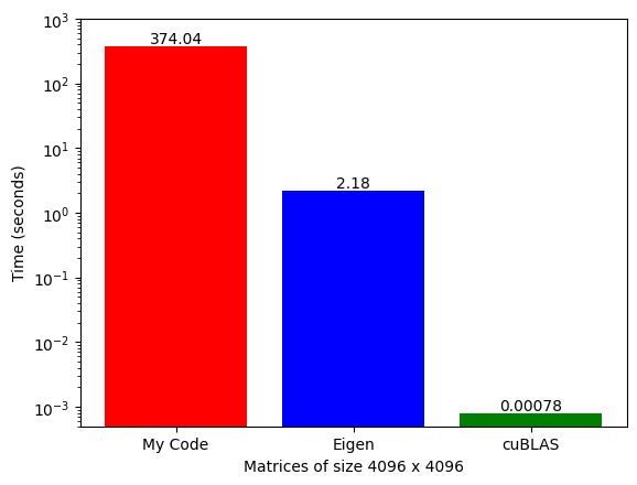
Figure 0.4: Naive CPU implementation vs Eigen implementation

Where NVIDIA shines is that it has developed a GPU-accelerated library called cuBLAS (that runs only on NVIDIA GPUs) and has a function called SGeMM (Single Precision General Matrix Multiplication) that can do the same thing extremely fast.

#include <cublas_v2.h>

int main(int argc, char const *argv[])
{
    // .
    // .
    // .

    // Generate square matrices d_A, d_B and d_C
    // .
    // .
    // .
    
    // Perform matrix multiplication: d_C = alpha*(d_A * d_B) + beta*d_C
    float alpha = 1;
    float beta = 0;
    cublasSgemm(handle,
                CUBLAS_OP_N, CUBLAS_OP_N,
                n, n, n, // Num Cols of C, Num rows of C, Shared dim of A and B
                &alpha,
                d_B, n, // Num cols of B
                d_A, n, // Num cols of A
                &beta,
                d_C, n // Num cols of C
              ); 

    // .
    // .
    // .

    return 0;
}

Matrix Multiplication using cuBLAS

Figure 0.5: Naive CPU vs Eigen vs cuBLAS

NVIDIA GPUs are the main reason for this speed-up. Whenever we write standard code in high-level programming languages like C++, by default, it runs sequentially on the CPU. We can exploit some level of parallelism from CPUs (that's what Eigen does), but GPUs are built specifically for parallel computing. NVIDIA provides CUDA (Compute Unified Device Architecture), allowing software to use GPUs for accelerated general-purpose processing.

💡

At first glance, 2.18 seconds might not look that bad. However, you have to understand that while training a neural network, matrix multiplication is performed millions of times. So even if we (very conservatively) assume 10 million matrix multiplications, it will take around 252 days to finish this on a CPU (using Eigen). While, on GPU that can be done in around 2 hours!

My goal with this mini project is to code general matrix multiplication from scratch in CUDA C++ and (try to) get as close as possible to the cuBLAS SGEMM implementation. I will do this step by step (keeping the code base as simple as possible) and, along the way, discuss:

CUDA API functions and how to use them.
NVIDIA GPU hardware, including CUDA cores and various memory units.
Several parallel GPU programming concepts like:
1. Global memory coalescing
2. 2D block tiling
3. 1D and 2D thread tiling
4. Vectorized memory accesses

Chapter 1: What is SGeMM

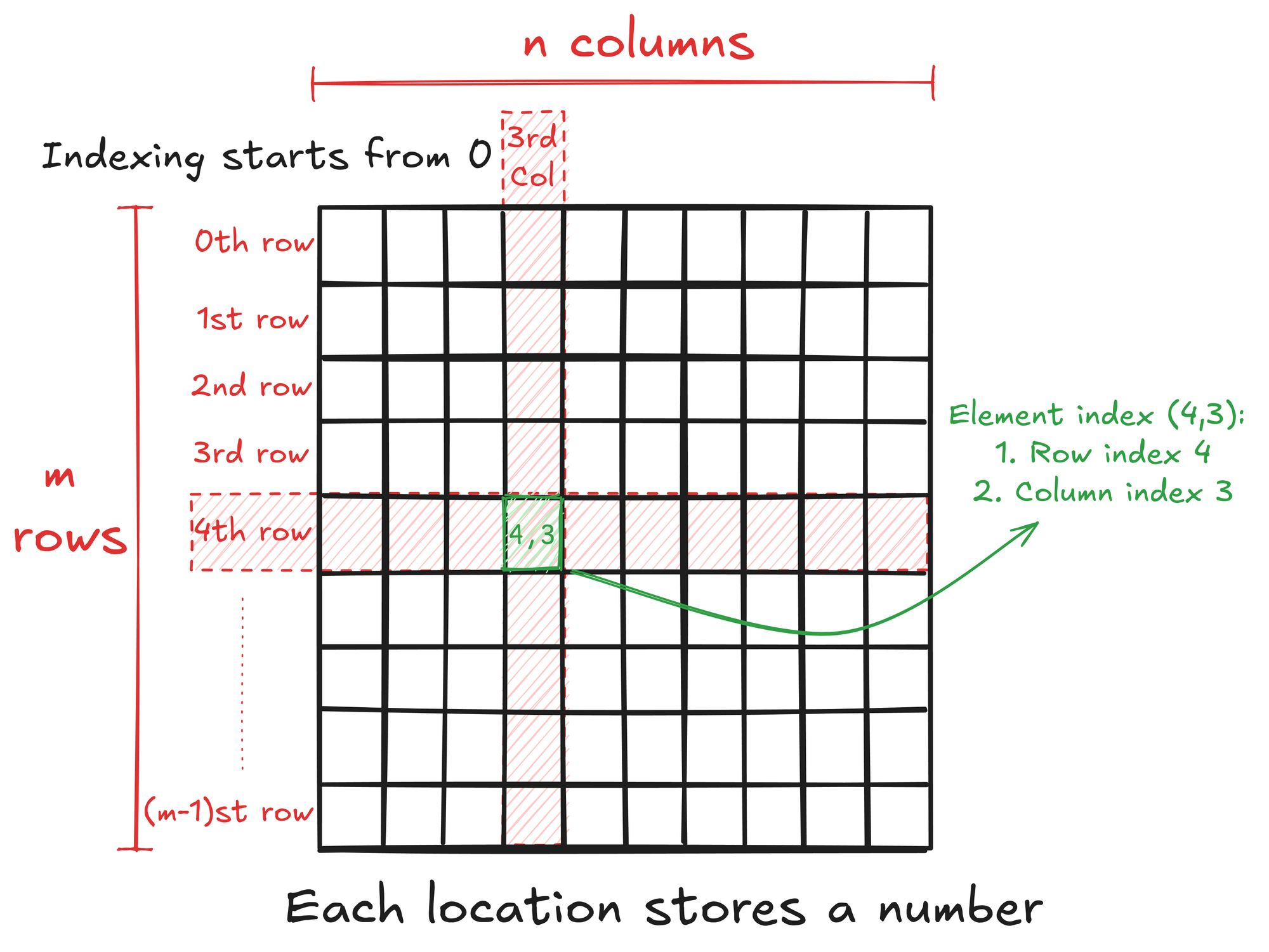
SGeMM stands for Single-Precision General Matrix Multiplication. A matrix is a rectangular array of numbers arranged in rows and columns. So, an M by N matrix (written as M x N) has M rows and N columns with a total of M x N numbers. The benefit of arranging numbers in a matrix is that it gives structure to the data, and we can easily access any number by specifying its location.

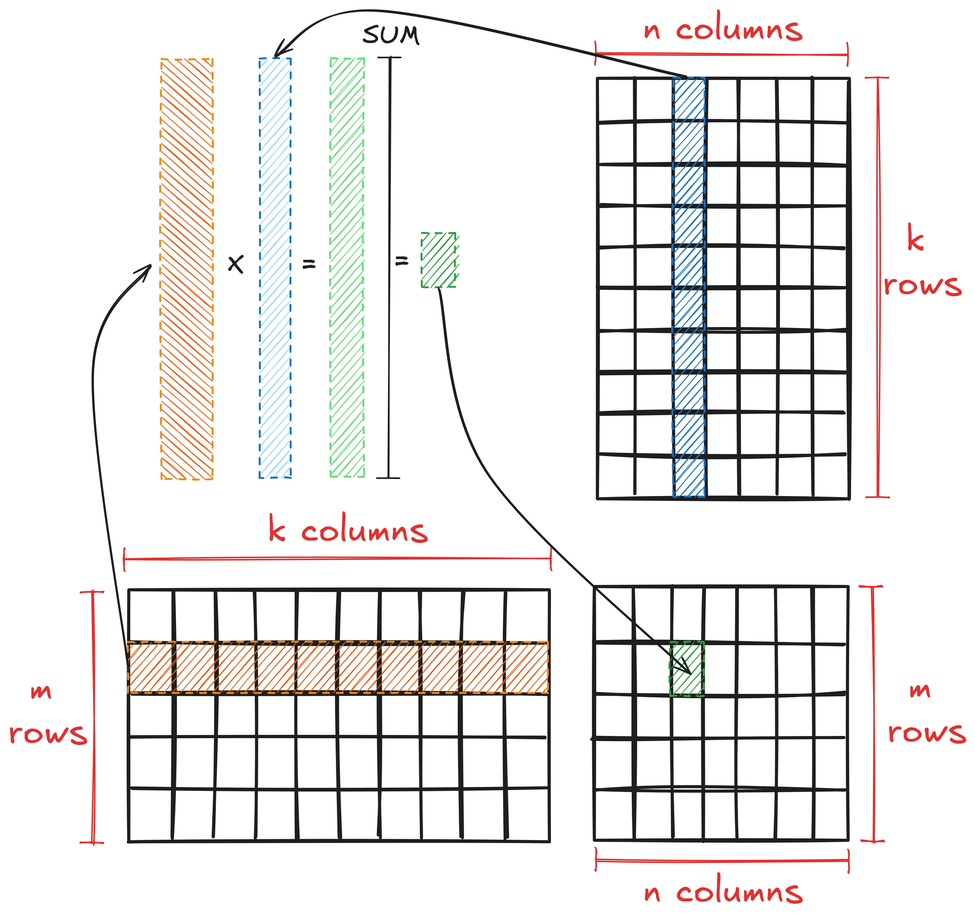
General matrix multiplication is a fundamental operation in linear algebra with specific rules and properties. Matrix multiplication is defined for two matrices A and B only when the number of columns in A is equal to the number of rows in B, i.e., if :

A is an M x K matrix
B is a K x N matrix
Then, their product AB is an M x N matrix.

To multiply matrices A and B:

Take each row of A and perform element-wise multiplication with each column of B.
The resulting elements are the sum of these multiplications.

Mathematically, this is expressed as:

$ \textbf{AB}_{ij} = \sum_{k=0}^{K-1} \textbf{A}_{i,k} \cdot \textbf{B}_{k,j} $

Where $\textbf{AB}_{ij}$ is the element in the i-th row and j-th column of the resulting matrix.

💡

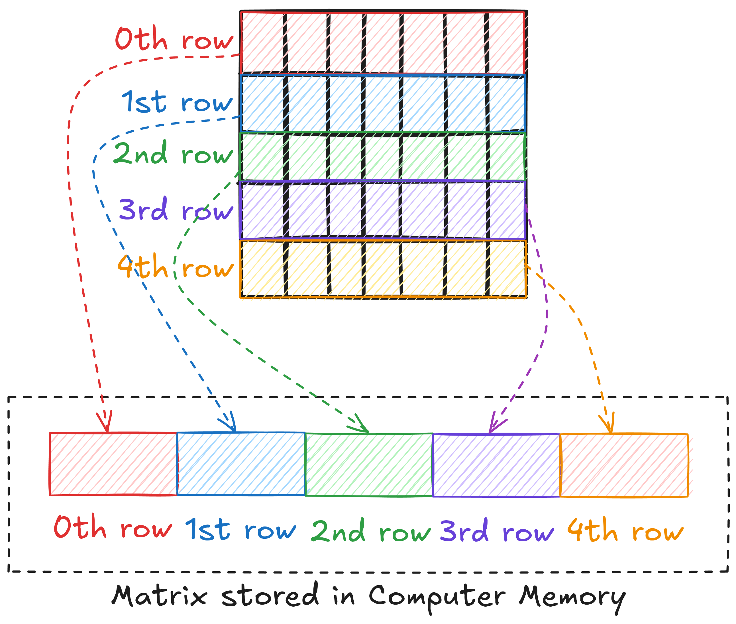
Figure 1.2 shows how an element of the output matrix is computed using a row and a column from input matrices. The same thing is done for all the other elements, and only the row and column from the input matrices change.

Matrices and Computer Memory

Computer memory is often presented as a linear address space through memory management techniques. This means that we cannot store a matrix in 2D form. Languages like C/C++ and Python store a 2D array of elements in a row-major layout, i.e., in the memory, 1st row is placed after the 0th row, 2nd row after 1st row, and so on.

Figure 1.3: Row major layout for storing matrices

💡

FORTRAN stores 2D arrays in column major layout.

This means that to access an element, we need to linearize the 2D index of the element. For example, if matrix A is M x N, the linearized index of element (6, 8) can be written as $6 \cdot N + 8$.

💡

Generally speaking, any element $(i, j)$ is at the location $i \cdot N + j$ in the memory.

So far, we have discussed matrices in general and the multiplication involving two matrices. Let's now look at what single-precision means.

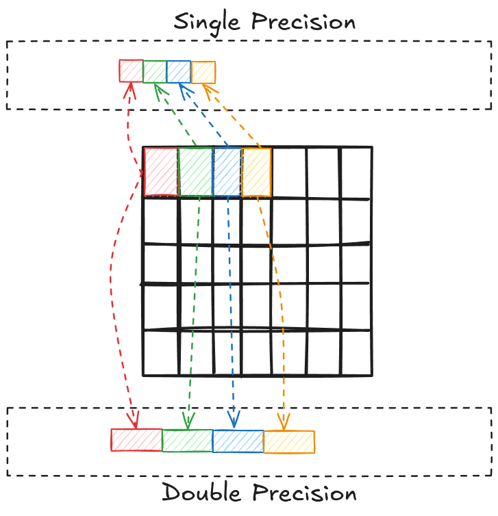
Memory Precision

The bit (binary digit) is the smallest and most fundamental digital information and computer memory unit. A byte is composed of 8 bits and is the most common unit of storage and one of the smallest addressable units of memory in most computer architectures. There are several ways to store the numbers in a matrix. The most common one is double precision (declared as double in C/C++). In double precision, a number is stored using 8 consecutive bytes in the memory. Another way is to store the numbers as a single precision type (declared as float in C/C++), where a number is stored using 4 consecutive bytes in the memory. This way, we can store the same number that takes up less space in memory, but we give up accuracy and the range of values we can work with.

💡

Single precision provides about 7 decimal digits of precision, and double precision provides about 15-17 decimal digits of precision. Single precision can represent numbers from approximately $1.4 \times 10^{-45}$ to $3.4 \times 10^{38}$, and double precision can represent numbers from approximately $4.9 \times 10^{-324}$ to $1.8 \times 10^{308}$.

NVIDIA uses single precision because it is generally preferred over double precision on GPUs for a few reasons:

Sufficient accuracy: For many graphics and scientific computing applications, single precision provides adequate accuracy while offering performance benefits.
Memory bandwidth: Single precision (4-byte) values require half the memory bandwidth of double precision (8-byte) values.
Computational units: GPUs typically have more single-precision computational units than double-precision units.
Throughput: Single-precision operations can be performed at a higher rate than double-precision operations.
Memory capacity: Using single precision allows more data to fit in the GPU's memory, reducing the need for data transfers between GPU and CPU memory.
Power efficiency: Single precision computations consume less power than double precision, allowing for better performance within thermal constraints.
Specialized hardware: Many GPUs have tensor cores or other specialized units optimized for single-precision or lower-precision (e.g., half-precision) calculations, particularly for AI/ML workloads.

💡

Half precision (2-bytes) floating point numbers are not natively supported in standard C++. However, we have an option to use half precision in CUDA (declared as half).

MatrixFP32

Matrix width is essential when linearizing a 2D index of an element. To avoid any mistakes (or confusion) while working with multiple matrices, I defined a simple (lightweight) class MatrixFP32, which keeps track of the float data pointer and the rows/columns of the matrix.

class MatrixFP32
{
public:
    const int n_rows;        // Number of rows
    const int n_cols;        // Number of cols

    // Pointer to dynamic array
    float* ptr;

    // Constructor to initialize n_rows x n_cols matrix
    MatrixFP32(int n_rows, int n_cols);
    
    // Free memory
    void free_mat();
};

MatrixFP32::MatrixFP32(int n_rows_, int n_cols_) : n_rows(n_rows_), n_cols(n_cols_)
{
    // Initialize dynamic array
    ptr = new float[n_rows*n_cols];
}

void MatrixFP32::free_mat()
{
    delete[] ptr;
}

This way, I can easily access any element of a matrix defined using MatrixFP32.

// Define an n x n matrix A_FP32
MatrixFP32 A_FP32 = MatrixFP32(n, n);

// Get element (4, 6)
float element = A_FP32.ptr[4*A_FP32.n_cols + 6];

Matrix Multiplication

The algorithm shown in Figure 1.2 can be written in C++ quite easily (in around 10 lines of code).

void cpu_xgemm(MatrixFP32 A_mat, MatrixFP32 B_mat, MatrixFP32 C_mat)
{
    // Getting A Matrix Dimension
    int A_n_rows = A_mat.n_rows; 
    int A_n_cols = A_mat.n_cols;

    // Getting B Matrix Dimension
    int B_n_rows = B_mat.n_rows; 
    int B_n_cols = B_mat.n_cols;

    // Getting C Matrix Dimension
    int C_n_rows = C_mat.n_rows; 
    int C_n_cols = C_mat.n_cols;

    // Asserting dimensions
    assert (A_n_cols == B_n_rows && "Matrices A & B must have one common dimension");
    assert (A_n_rows == C_n_rows && "A rows must be equal to C rows");
    assert (B_n_cols == C_n_cols && "B cols must be equal to C cols");

    // Matrix Multiplication
    for (int row = 0; row < A_n_rows; row++)
    {
        for (int col = 0; col < B_n_cols; col++)
        {
            float val = 0.0f;
            for (int k = 0; k < A_n_cols; k++)
            {
                val += A_mat.ptr[row*A_n_cols + k] * B_mat.ptr[k*B_n_cols + col];
            }
            C_mat.ptr[row*C_n_cols + col] = val;
        }
    }
}

Sequential matrix multiplication on a CPU

By looking at this code, we can sense that the algorithm might be computationally intensive (3 nested loops!). Figure 1.5 plots the time to perform matrix multiplication using this code for matrix sizes ranging from 128 to 4096. We can see that the growth is somewhat exponential as the matrix size increases (technically, it's around $n^3$).

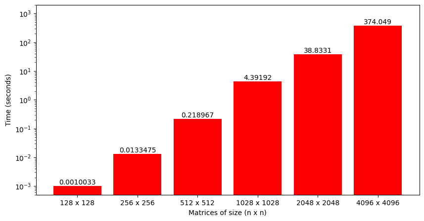
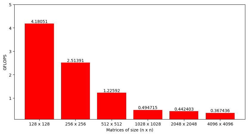
Figure 1.5: Runtime for sequential matrix multiplications on a CPU

💡

With 1024x increase in the number of elements (from 128 x 128 to 4096 x 4096), execution time increases 3728186x!

Even though time is a perfectly fine metric to analyze, a better option is to look at the number of operations performed per second by the function or Giga Floating-Point Operations per second (GFLOPS). When multiplying two M x K and K x N, each output matrix element requires approximately K multiplications and K additions, i.e., 2K operations. As there are total M x N output elements, the total number of operations is 2 x M x N x K. Dividing this number by the time it took to perform matrix multiplication gives FLOPS for the implemented algorithm (that can be converted to GFLOPS).

Figure 1.6: GFLOPS for sequential matrix multiplications on a CPU

💡

Figures 1.5 and 1.6 show the same thing essentially, but GFLOPS is a more general metric that takes algorithm complexity into account as well, and I will be using this moving forward.

Fortunately, matrix multiplication can be parallelized quite efficiently. The next step is understanding how this algorithm can be parallelized and then implementing a basic parallel matrix multiplication that runs on the GPU.

To get a taste of the power of GPUs, CUDA provides a function SGEMM that can do this in a single line of code. To be more precise, the SGEMM function performs $C = \alpha A \cdot B + \beta C$ (i.e., matrix multiplication and accumulation). However, we can set $\alpha=1$ and $\beta=0$ to just get matrix multiplication.

// Perform matrix multiplication: C = A * B 
float alpha = 1;
float beta = 0;
cublas_check(cublasSgemm(handle,
                        CUBLAS_OP_N, CUBLAS_OP_N,
                        d_C_FP32.n_cols, d_C_FP32.n_rows, d_A_FP32.n_cols, // Num Cols of C, Num rows of C, Shared dim of A and B
                        &alpha,
                        d_B_FP32.ptr, d_B_FP32.n_cols, // Num cols of B
                        d_A_FP32.ptr, d_A_FP32.n_cols, // Num cols of A
                        &beta,
                        d_C_FP32.ptr, d_C_FP32.n_cols) // Num cols of C
            );

Figure 1.7: GFLOPS for parallel matrix multiplications on a GPU using cuBLAS

Chapter 2: Getting Started with CUDA Programming

If we look at the matrix multiplication algorithm carefully (Figure 2.1), it's obvious that each output matrix element can be computed independently. Each output element requires a unique combination of row and column of the input matrices, and most importantly, one output element does not depend on any other output element.

Figure 2.1: Matrix multiplication algorithm

void cpu_xgemm(MatrixFP32 A_mat, MatrixFP32 B_mat, MatrixFP32 C_mat)
{
    // Getting A Matrix Dimension
    int A_n_rows = A_mat.n_rows; 
    int A_n_cols = A_mat.n_cols;

    // Getting B Matrix Dimension
    int B_n_rows = B_mat.n_rows; 
    int B_n_cols = B_mat.n_cols;

    // Getting C Matrix Dimension
    int C_n_rows = C_mat.n_rows; 
    int C_n_cols = C_mat.n_cols;

    // Asserting dimensions
    assert (A_n_cols == B_n_rows && "Matrices A & B must have one common dimension");
    assert (A_n_rows == C_n_rows && "A rows must be equal to C rows");
    assert (B_n_cols == C_n_cols && "B cols must be equal to C cols");

    // Matrix Multiplication
    for (int row = 0; row < A_n_rows; row++)
    {
        for (int col = 0; col < B_n_cols; col++)
        {
            float val = 0.0f;
            for (int k = 0; k < A_n_cols; k++)
            {
                val += A_mat.ptr[row*A_n_cols + k] * B_mat.ptr[k*B_n_cols + col];
            }
            C_mat.ptr[row*C_n_cols + col] = val;
        }
    }
}

Sequential matrix multiplication on a CPU

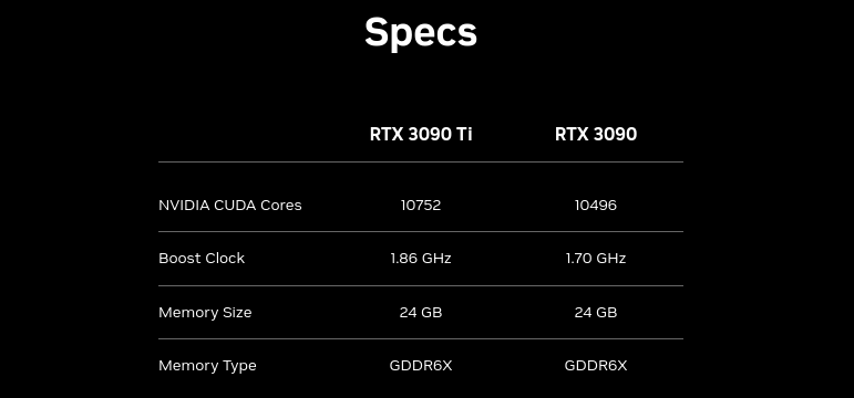
This means we can parallelize loops row and col and reduce the computation cost significantly. GPUs are designed specifically for problems like this. Figure 2 shows a screenshot from NVIDIA's website. The first thing they mention about their GPUs is the number of CUDA cores. CUDA cores are the basic computational units in NVIDIA GPUs that handle parallel processing tasks.

💡

There is a lot more to a GPU than the number of cores and we will discuss other details whenever they are necessary. The last thing I want to do is overwhelm with details at the very start and lose sight of the goal.

CPU and GPU

CPUs and GPUs have execution units (called cores) that perform the arithmetic operations and an off-chip memory unit (RAM and VRAM, respectively) to store the required data. The big difference is that a CPU has much fewer cores than a GPU.

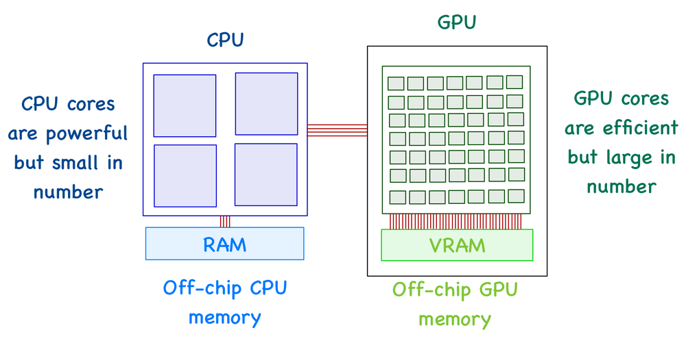
A GPU can't function independently. It's the job of a CPU to move data between RAM and VRAM (or global memory). In other words, a CPU can be seen as an instructor who manages most of the tasks and is responsible for assigning specific tasks to the GPU (where it has an advantage).

On the software side of things, we don't control the processing units. Instead, the hardware spawns threads, which a programmer can work with. A thread can be seen as an individual worker, and the execution of a thread is sequential as far as a user is concerned, i.e., a worker can only do one task at a time, but we can have multiple workers that can all work in parallel.

💡

Threads are at the heart of modern computing. A thread is a simplified view of how a processor executes a sequential program in modern computers.

GPUs are suited for parallel programming because the hardware can spawn millions of threads (way more than the number of physical cores). Conversely, CPUs can only generate a handful of threads (~8 to 128).

GPU Programming Model

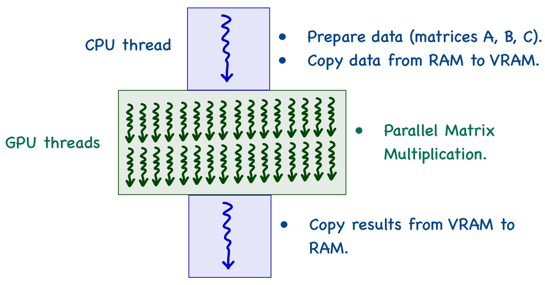
When we write a program in a high-level language like C/C++, by default, the CPU execution uses a single thread. All the matrices are on RAM (at this point), and the CPU thread copies the data to global memory. The GPU can then spawn multiple threads that work in parallel to reduce computation time. Once the execution finishes, the CPU thread copies the results from global memory to RAM.

A CPU thread can't just copy data straight away. The first step is to allocate the exact amount of memory required to global memory. It is done using cudaMalloc function (which is provided by CUDA). This function accepts two parameters:

The first parameter is the address of the pointer variable for the select matrix. The address of this pointer must be cast (void **) because the function expects a generic pointer (not restricted to a specific type).
The second parameter is the size of the data to be allocated (in number of bytes).

// Device array pointers for N x N matrix
float* d_A;

// Device memory allocation
cudaError_t err_A = cudaMalloc((void**) &d_A, N*N*sizeof(float));
// CUDA error checking code (see code repository for more details)
CUDA_CHECK(err_A);

💡

The first parameter is the address of the pointer because this allows the cudaMalloc function to return a value (of type cudaError_t) reporting errors during global memory allocation (which can then be passed to the CUDA error-checking code).

As I'm using a custom class MatrixFP32 to handle matrices, I can embed the above mentioned code such that global memory gets allocated whenever an object destined for GPU is created. To do this, I made two modifications:

Added a member variable on_device that keeps track of whether the object is destined for CPU or GPU memory (this is set to true for the GPU).
Added a separate initialization/memory allocation code for global memory in the constructor and modified the free_mat method appropriately.

class MatrixFP32
{
public:
    const int n_rows;        // Number of rows
    const int n_cols;        // Number of cols

    // Pointer to dynamic array
    float* ptr;
    
    // Matrix in device memory: true; else: false
    const bool on_device; 
    
    // Constructor to initialize n_rows x n_cols matrix
    MatrixFP32(int n_rows_, int n_cols_, bool on_device);
    
    // Free memory
    void free_mat();
};

MatrixFP32::MatrixFP32(int n_rows_, int n_cols_, bool on_device_) : n_rows(n_rows_), n_cols(n_cols_), on_device(on_device_)
{
    if (on_device_ == false)
    {
        // Initialize dynamic array
        ptr = new float[n_rows*n_cols];
    }
    else
    {
        // Allocate device memory
        cudaError_t err = cudaMalloc((void**) &ptr, n_rows*n_cols*sizeof(float));
        cuda_check(err);
    }
}

void MatrixFP32::free_mat()
{
    if (on_device == false)
        delete[] ptr;
    else
        cudaFree(ptr);
}

Once the memory has been allocated in the global memory, data can be transferred between RAM and global memory using cudaMemcpy function. This function accepts four parameters:

Pointer to the destination
Pointer to the source
Number of bytes to be copied
The direction of transfer:
- When copying data from RAM to global memory, this will be cudaMemcpyHostToDevice
- When copying data from global memory to RAM, this will be cudaMemcpyDeviceToHost
- Note that these are symbolic predefined constants of the CUDA programming environment.

// Copying A to device memory
cudaError_t err_A_ = cudaMemcpy(d_A, A, N*N*sizeof(float), cudaMemcpyHostToDevice);
CUDA_CHECK(err_A_);

// Copy C to host memory
cudaError_t err_C_ = cudaMemcpy(C, d_C, N*N*sizeof(float), cudaMemcpyDeviceToHost);
CUDA_CHECK(err_C_);

💡

In accelerator language, host refers to the CPU and device is the accelerator, here the GPU.

I added two more methods to the class that can copy data between CPU and GPU (while checking the size compatibility and other details) to automate much of this stuff.

void MatrixFP32::copy_to_device(MatrixFP32 d_mat)
{
    // Make sure that ptr is on host 
    assert(on_device == false && "Matrix must be in host memory");
    assert(d_mat.on_device == true && "Input Matrix to this function must be in device memory");

    // Copying from host to device memory
    cudaError_t err = cudaMemcpy(d_mat.ptr, ptr, n_rows*n_cols*sizeof(float), cudaMemcpyHostToDevice);
    cuda_check(err);
}

void MatrixFP32::copy_to_host(MatrixFP32 h_mat)
{
    // Make sure that ptr is on device
    assert(on_device == true && "Matrix must be in device memory");
    assert(h_mat.on_device == false && "Input Matrix to this function must be in host memory");

    // Copying from host to device memory
    cudaError_t err = cudaMemcpy(h_mat.ptr, ptr, n_rows*n_cols*sizeof(float), cudaMemcpyDeviceToHost);
    cuda_check(err);
}

This allows us to easily transfer data between CPU and GPU with very few visible lines of code.

// Define MatrixFP32
MatrixFP32 A_FP32 = MatrixFP32(n, n, false);
MatrixFP32 B_FP32 = MatrixFP32(n, n, false);
MatrixFP32 C_FP32 = MatrixFP32(n, n, false);

// Initialize Matrix
// .
// .
// .

// Move matrix to device
MatrixFP32 d_A_FP32 = MatrixFP32(n, n, true); 
A_FP32.copy_to_device(d_A_FP32);

MatrixFP32 d_B_FP32 = MatrixFP32(n, n, true); 
B_FP32.copy_to_device(d_B_FP32);

MatrixFP32 d_C_FP32 = MatrixFP32(n, n, true); 
C_FP32.copy_to_device(d_C_FP32);

// Perform computations on GPU
// .
// .
// .

// Copy results to host
d_C_FP32.copy_to_host(C_FP32);

// Free Memory
A_FP32.free_mat();
B_FP32.free_mat();
C_FP32.free_mat();

d_A_FP32.free_mat();
d_B_FP32.free_mat();
d_C_FP32.free_mat();

Parallel Matrix Multiplication

Now that the data transfer is all taken care of let's see how we can program the GPU to perform matrix multiplication in parallel. The algorithm for parallel matrix multiplication involving matrix A of size (M x K) and B of size (K x N) is as follows:

$M \cdot N$ threads are generated on the GPU (one to compute each element of the matrix $C$, which is of size M x N).
Each thread:
1. Retrieves a row of matrix $A$ and a column of matrix $B$.
2. Loops over the elements.
3. Multiplies the two numbers and add the result to the total.

Figure 2.5: Parallel Matrix Multiplication

Now, who decides which thread works on which element of the matrix $C$? We need to understand how threads are organized on a GPU to answer this question.

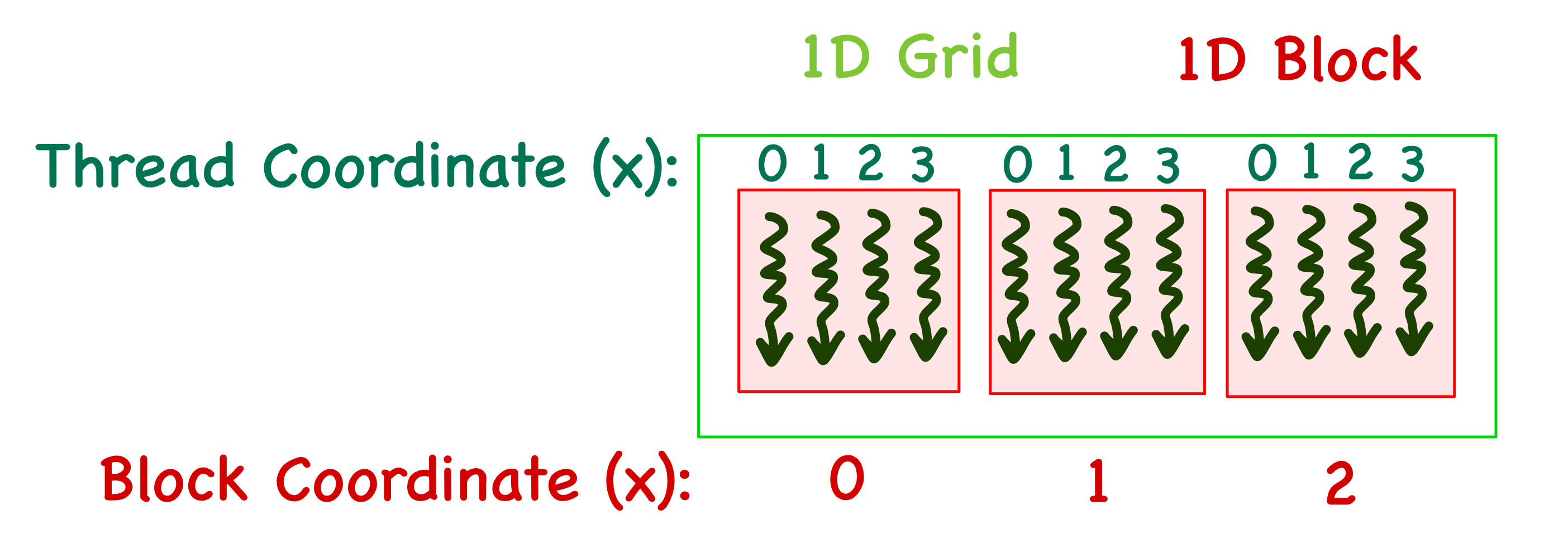
When the kernel function is called, it creates a grid of threads on the GPU. The grid is subdivided into multiple blocks, each containing the same amount of threads. The blocks in a grid and threads in a block can be arranged in a 1D/2D/3D manner with coordinates (x,y,z) assigned to the blocks and the threads inside each block.

The 1D case is the simplest, with only an x index. For example, consider a grid with 3 blocks and 4 threads in each block. The blocks will then have x coordinates ranging from 0 to 2, and threads in each block will have x coordinates ranging from 0 to 3. It is important to note that each block's thread index is local.

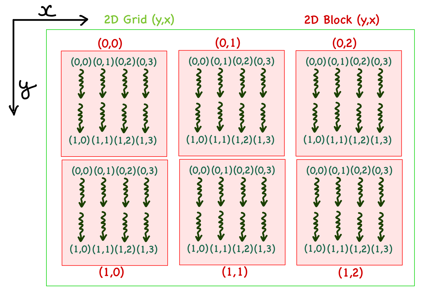
In the 2D case, there are x and y indices. For example, consider a grid with 3 blocks in x direction and 2 blocks in y direction. Each block has 4 and 2 threads in the x and y directions. In the case of a 2D organization, it is important to note that the y index precedes x, i.e., it's written as (y,x) such that y is for the vertical direction and x is for the horizontal.

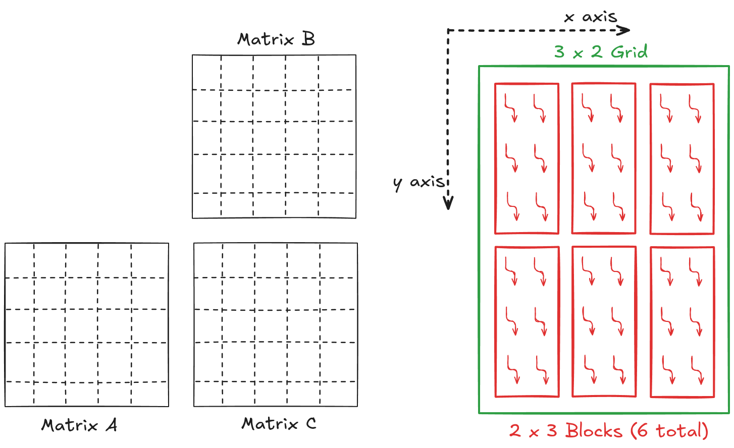
For example, consider matrix multiplication involving 5 x 5 matrices ($C = A \cdot B$). Let's define a 2 x 3 block to perform matrix multiplication in parallel. We need a 3 x 2 grid to cover all the output matrix elements.

Threads shown in Figure 2.8 have local indices similar to the ones shown in Figure 2.7. We can calculate a global index for each thread using these local and block indices. This global index is nothing but a unique index for each thread.

$$\text{Global x} = \text{blockDim}.x \cdot \text{blockIdx}.x + \text{threadIdx}.x$$
$$\text{Global y} = \text{blockDim}.y \cdot \text{blockIdx}.y + \text{threadIdx}.y$$

blockDim.x and blockDim.y are the number of blocks in x and y axis respectively.
blockIdx.x and blockIdx.y are the block index in x and y axis respectively.
threadIdx.x and threadIdx.y are the thread index in x and y axis respectively.

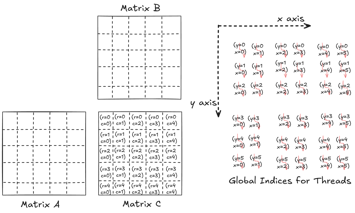
Figure 2.9 shows the global indices for all the threads alongside the row and column indices for the element of matrix C. One way to solve this in parallel is to match the thread's x index with the row index and y with the column index.

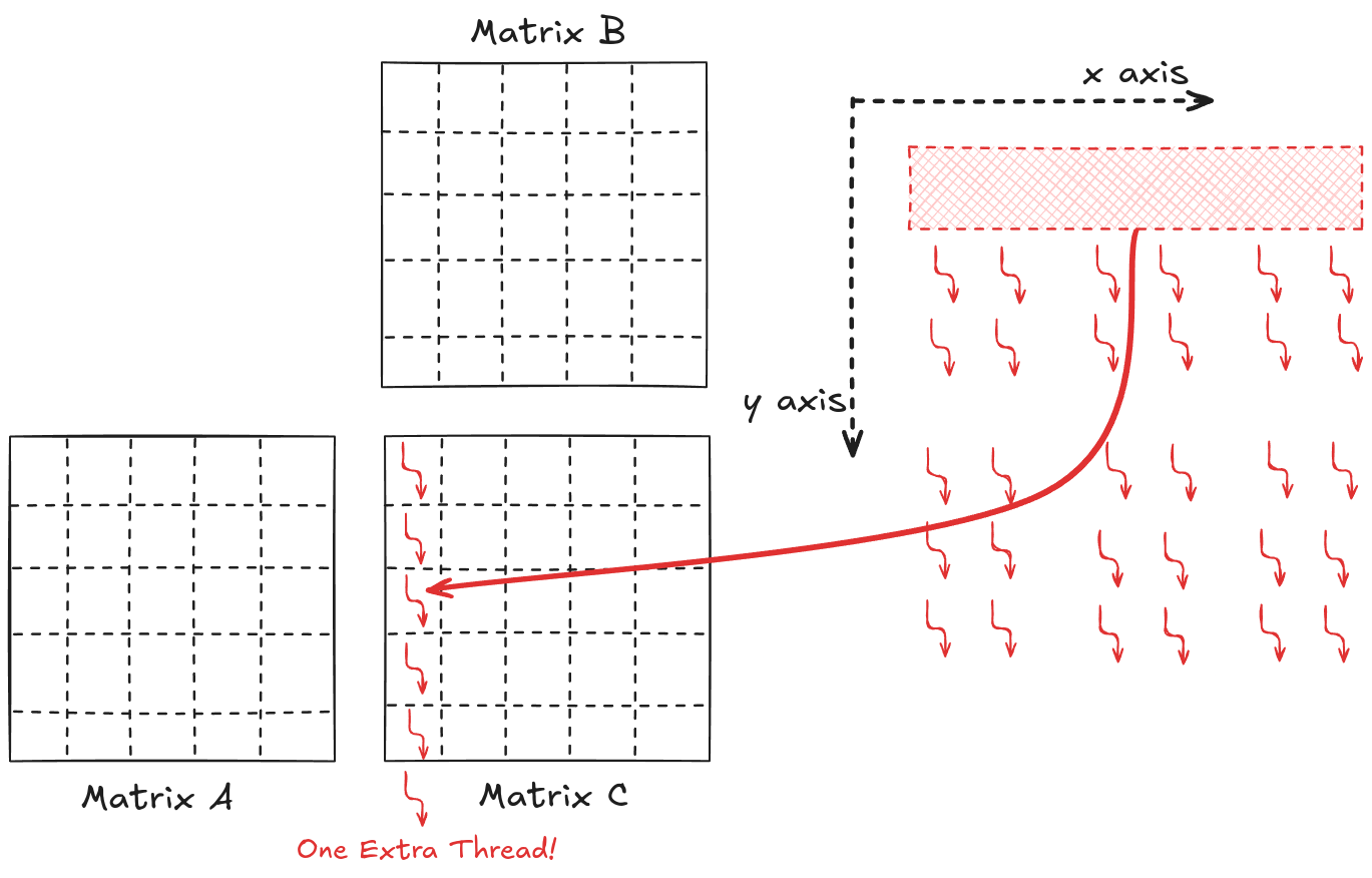
Figure 2.10 shows the thread-to-element mapping for the 1st column of the elements of C. The same procedure will map the rest of the elements to the threads (Figure 11). Note that there are additional threads that map to non-existent elements. This is common, and in code, we can make sure that these threads stay idle.

Figure 2.11: Animation showing thread to element mapping

Looking back at the general case for parallel matrix multiplication involving matrix A of size (M x K) and B of size (K x N), the resulting matrix C will be M x N. The first thing we need to decide is the dimensionality of the block (i.e., the number of threads and their organization in a block). CUDA restricts the total number of threads in a block can't be more than 1024. This means that the organization can be (512,1,1) or (8,16,4) (just as long as the total number is not greater than 1024). As an example, let's go with (32, 32). Based on this, we can determine the total number of blocks required in the x and y dimensions.

The custom-defined CUDA type dim3 defines

The number of threads in each block: dim3 dim_block(32, 32, 1). Note that in this case, the z dimension is set to 1.
The number of blocks in the grid can then be decided based on the matrix size and the total threads in each block: dim3 dim_grid(ceil(C_n_rows/32.0), ceil(C_n_cols/32.0), 1);.

void naive_xgemm(float *d_A_ptr, float *d_B_ptr, float *d_C_ptr, int C_n_rows, int C_n_cols, int A_n_cols)
{
    // Kernel execution
    dim3 dim_block(32, 32, 1);
    dim3 dim_grid(ceil(C_n_rows/(float)(32)), ceil(C_n_cols/(float)(32)), 1);
    //.
    //.
    //.
}

Now that a grid of threads is defined, the next step is to code the instructions these threads need to execute. This is done with the kernel function. It is a normal-looking function that each thread executes independently. In short, all the threads perform the same instructions. The only difference between different threads is the data these instructions are performed on. As all the threads access the same function, we can use the local indices to compute the global index and then perform the necessary calculations.

__global__ void naive_mat_mul_kernel(float *d_A_ptr, float *d_B_ptr, float *d_C_ptr, int C_n_rows, int C_n_cols, int A_n_cols)
{
    // Working on C[row,col]
    const int row = blockDim.x*blockIdx.x + threadIdx.x;
    const int col = blockDim.y*blockIdx.y + threadIdx.y;

    // Parallel mat mul
    if (row < C_n_rows && col < C_n_cols)
    {
        // Value at C[row,col]
        float value = 0;
        for (int k = 0; k < A_n_cols; k++)
        {
            value += d_A_ptr[row*A_n_cols + k] * d_B_ptr[k*C_n_cols + col];
        }

        // Assigning calculated value (SGEMM is C = α*(A @ B)+β*C and in this repo α=1, β=0)
        d_C_ptr[row*C_n_cols + col] = 1*value + 0*d_C_ptr[row*C_n_cols + col];
    }
}

💡

Notice how there is no loop in the kernel function. Instead, each thread replaces a loop iteration and operates in parallel to other threads. __global__ is a qualifier keyword that suggests this function is callable from the host and can only be executed on the device.

The final step is to launch this kernel function so that all the threads execute it. This is done by specifying the grid organization inside <<< >>> and passing the device variables.

void naive_xgemm(float *d_A_ptr, float *d_B_ptr, float *d_C_ptr, int C_n_rows, int C_n_cols, int A_n_cols)
{
    // Kernel execution
    dim3 dim_block(32, 32, 1);
    dim3 dim_grid(ceil(C_n_rows/(float)(32)), ceil(C_n_cols/(float)(32)), 1);
    naive_mat_mul_kernel<<<dim_grid, dim_block>>>(d_A_ptr, d_B_ptr, d_C_ptr, C_n_rows, C_n_cols, A_n_cols);
}

Benchmark

Chapter 3: GPU Global Memory Coalescing

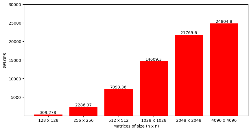
Looking at the GFLOPS from our kernel function and cuBLAS SGEMM (Figure 3.1), there are two main questions:

Why are GFLOPS increasing with matrix sizes?
How can we improve the performance of our kernel function?

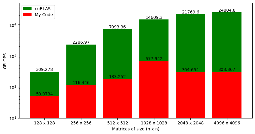
To answer these questions, we need to understand the GPU hardware better.

Modern GPU Architecture

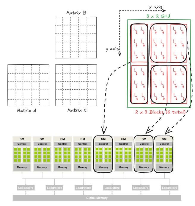
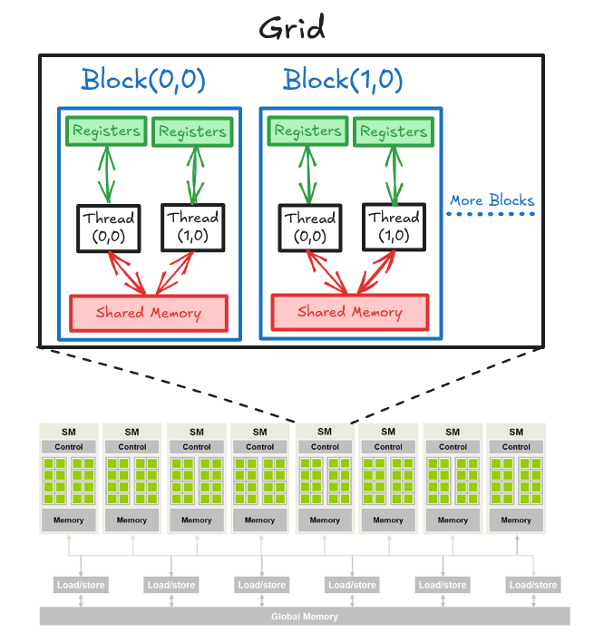
Figure 3.2 shows a high-level CUDA C programmer's view of a CUDA-capable GPU's architecture. There are four key features in this architecture:

The GPU is organized into an array of highly threaded streaming multiprocessors (SMs).
Each SM has several processing units called streaming processors or CUDA cores (shown as green tiles inside SMs) that share control logic.
The SMs also contain a different on-chip memory shared amongst the CUDA cores inside the SM.
GPU also has a much larger off-chip memory, the main component of which is the global memory or VRAM.

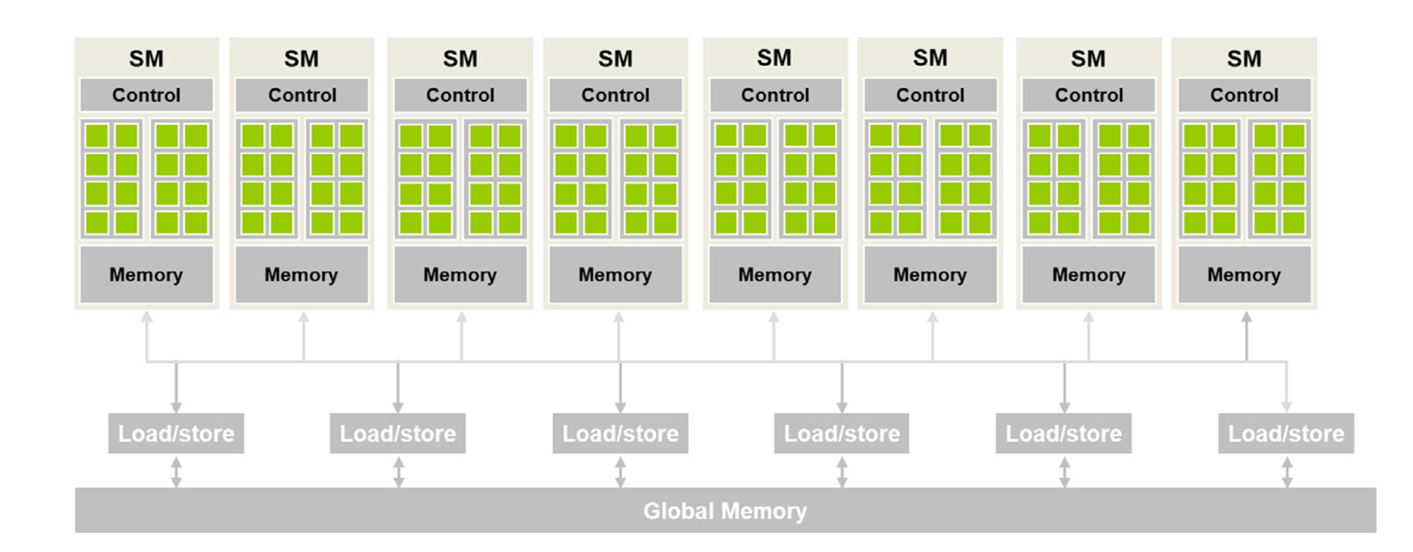
Figure 3.2: Architecture of a CUDA-capable GPU

There are two main takeaways from Figure 3.2:

CUDA cores in different SMs can't interact with each other or access memory from other SMs.
The global memory is off-chip (i.e., some distance away from the cores), so it has long latency and low bandwidth.

💡

Latency is the time it takes for data to travel from one point to another, usually measured in milliseconds (ms). Bandwidth is the maximum amount of data that can be sent and received in a given time, usually measured in Mbps or Gbps.

Thread Blocks and SMs

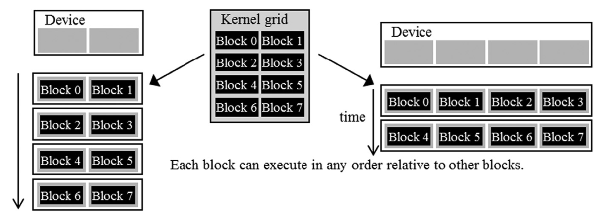
When a kernel is called, the CUDA runtime system launches a grid of threads that execute the same kernel code. These threads are assigned to SMs on a block-by-block basis, i.e., all threads in a block are simultaneously assigned to the same SM. For the matrix multiplication example, multiple blocks will likely get simultaneously assigned to the same SM.

The example discussed in Figure 3.3 is quite small. In real-world problems, there are a lot more blocks, and to ensure that all blocks get executed, the runtime system maintains a list of blocks that did not get assigned to any SM and assigns these new blocks to SMs when previously assigned blocks complete execution. This block-by-block assignment of threads guarantees that threads in the same block are executed simultaneously on the same SM, which makes interaction between threads in the same block possible.

For a moment, it might look like an odd choice not to let threads in different blocks interact with each other. However, this feature allows different blocks to run independently in any order, resulting in transparent scalability where the same code can run on different hardware with different execution resources. This, in turn, reduces the burden on software developers and ensures that with new generations of hardware, the application will speed up consistently without errors.

Figure 3.4: A Smaller GPU (on the left) can only run 2 blocks concurrently, while a larger GPU (on the right) can run 4 blocks concurrently.

Warps

In the previous section, I explained that blocks can execute in any order relative to each other, but I did not say anything about how threads inside each block are executed. Conceptually, the programmer should assume that threads in a block can execute in any order, and the correctness of the algorithm should not depend on the order in which threads are executed.

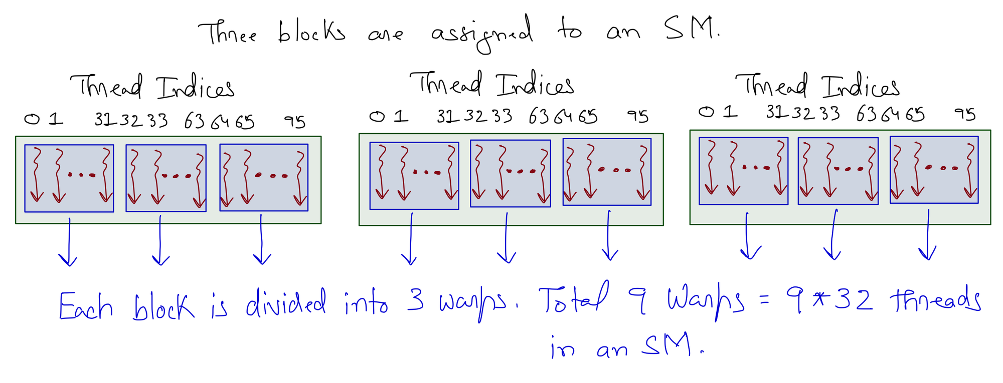
Thread scheduling in CUDA GPUs is a hardware implementation concept that varies depending on the type of hardware used. In most implementations, once a block is assigned to an SM, it is divided into 32-thread units called warps. The knowledge of warps is useful for understanding and optimizing the performance of CUDA applications.

💡

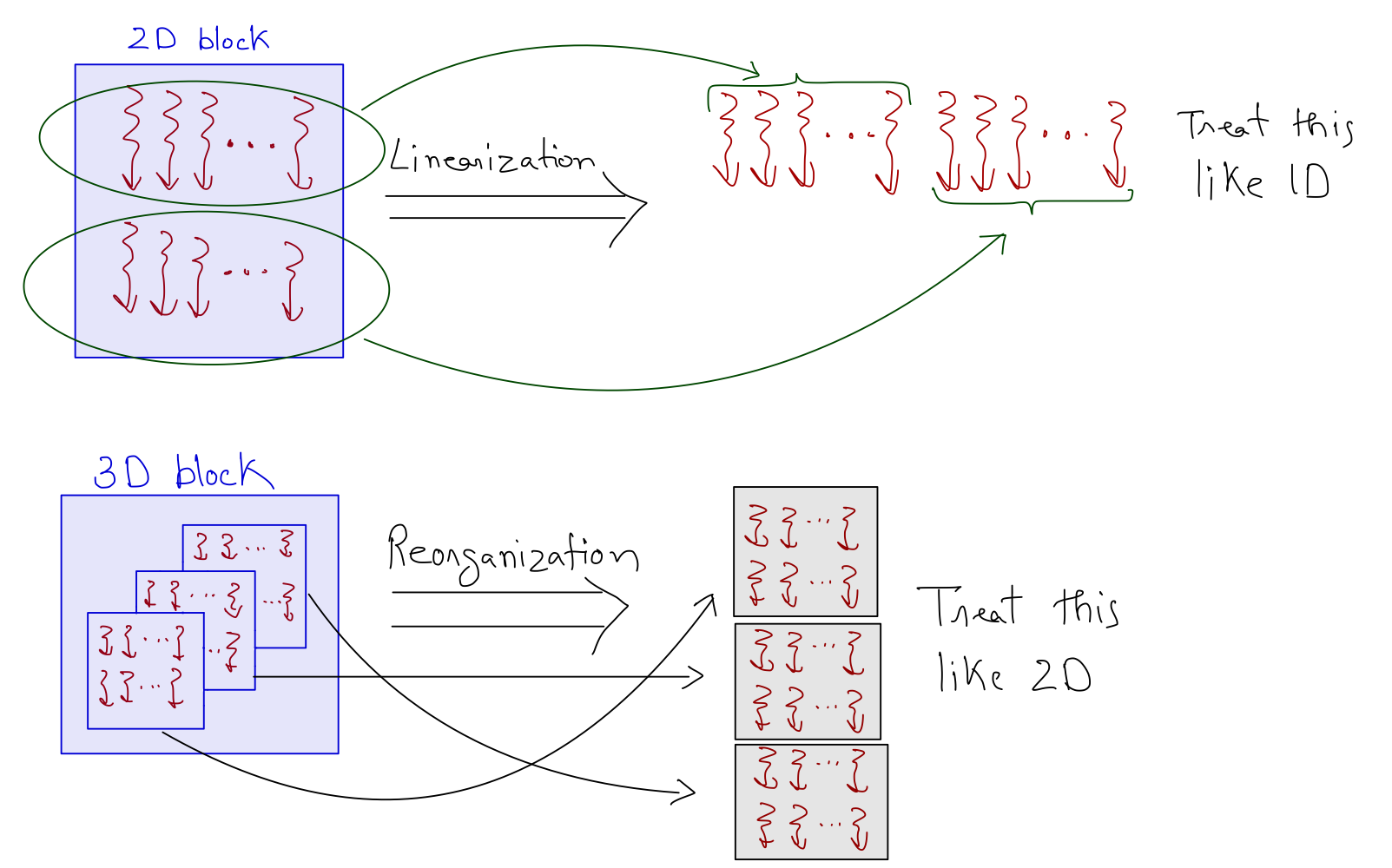
Warp size can be different for future hardware generations!

Each warp consists of 32 consecutive threads. For 1D block, this is straightforward such that threadIdx.x is used to divide the threads into warps.

💡

If the number of threads in a block is not a multiple of 32, the last warp gets padded with inactive threads to fill up the remaining thread positions.

For the 2D block, threads are linearized using a row-major layout and partitioned into warps like the 1D case. For the 3D block, the z dimension is folded into the y dimension, and the resulting thread layout is treated as the 2D case.

An SM is designed to execute all threads in a warp following the SIMD model, i.e., at any instance in time, one instruction is fetched and executed for all threads in the warp. As one instruction is shared across multiple execution units, it allows for a small percentage of the hardware to be dedicated to control, and a large percentage is dedicated to increasing the arithmetic throughput (i.e., cores).

Kernel Function

There are three main steps to running a program on the GPU:

Copy data from host memory to device global memory.
Perform computations using the device cores and the data stored in global memory.
Copy results from global memory to host memory.

We can't do much about steps 1 and 3 as we have to move data between host and device memory. To be honest, this is computationally intensive, but again, it's a one-time thing, and with large data, we can offset the cost with gains from solving the problem in parallel. So, my focus here is to analyze the kernel function.

As a recap, the algorithm for parallel matrix multiplication involving matrix A of size (M x K) and B of size (K x N) is as follows:

$M \cdot N$ threads are generated on the GPU (one to compute each element of the matrix $C$, which is of size M x N).
Each thread:
1. Retrieves a row of matrix $A$ and a column of matrix $B$ from the device memory. This results in 2 x 4K Bytes being copied from the device's global memory.
2. Loops over the elements.
3. Multiplies the two numbers and adds the result to the total stored in the device's global memory. This results in 4 Bytes being copied to the device memory.

For all M x N threads, we are accessing M x N x (2 x 4K + 4) Bytes. If we have 4096 x 4096 matrices, the accesses from global memory amount to 512 GB! I'm focusing so much on these memory accesses because global memory has long latency and low bandwidth, which is usually a major bottleneck for most applications.

Answering the Questions

Why does GFLOPS increase with increasing Matrix Size?

From the knowledge of the GPU hardware (that we have acquired so far), the loss in performance for matrix multiplication with small matrix sizes (Figure 1) is mostly due to the global memory accesses. However, this does not explain why GFLOPS increases with the increase in the matrix size. I mean that with large matrices, the number of global memory accesses also increases, but the performance increases counterintuitively! GPUs can do this because of the hardware latency tolerance or latency hiding.

There are usually more threads assigned to an SM than its cores. This is done so that GPUs can tolerate long-latency operations (like global memory accesses). With enough warps, SM can find a warp to execute while others are waiting for long-latency operations (like getting data from global memory). Filling the latency time of operations from some threads with work from others is called latency tolerance or latency hiding. The selection of warps ready for execution does not introduce any computational cost because GPU hardware is designed to facilitate zero-overhead thread scheduling.

💡

This context-switching can also be done with CPU threads. In CPUs, before switching to a different thread, the current execution state is moved from registers to memory and later loaded back to registers (from memory). This saving and restoring contents in a CPU can incur significant overhead.

💡

GPUs perform context switching differently, such that the execution state is held in place (inside thread registers). The ability to tolerate such long latency operations is why GPUs have smaller cache memories and control logic but way more registers. Another distinction from CPU is that GPU registers are not designed to store data but act as a staging area for threads.

That's why, for large matrices, more warps are available to hide the latency due to global memory accesses. There is a limit (set by CUDA) to the number of warps that can be assigned to an SM. However, it's impossible to assign an SM with the maximum number of warps it supports because of constraints on execution resources (like on-chip memory) in an SM. The resources are dynamically partitioned such that SMs can execute many blocks with few threads or a few blocks with many threads.

For example, an Ampere A100 GPU can support 32 blocks per SM, 64 warps (2048 threads) per SM, and 1024 threads per block

So, if

A grid is launched with 1024 threads in a block (maximum allowed)

Ans. Each SM can accommodate 2 blocks (with 2048 threads total, matching the maximum allowed per SM).

A grid is launched with 512 threads in a block

Ans. Each SM can accommodate 4 blocks (with 2048 threads total, matching the maximum allowed per SM).

A grid is launched with 256 threads in a block

Ans. Each SM can accommodate 8 blocks (with 2048 threads total, matching the maximum allowed per SM).

A grid is launched with 64 threads in a block

Ans. Each SM can accommodate 32 blocks (with 2048 threads total, matching the maximum allowed per SM).

💡

The ratio of the number of warps assigned to an SM to the maximum number it supports is known as occupancy.

A negative situation might arise when the maximum number of threads allowed per block is not divisible by the block size. For example, we know that an Ampere A100 GPU can support 2048 threads per SM

So, if

A grid is launched with 700 threads in a block

Ans. SM can hold only 2 blocks (totaling 1400 threads), and the remaining 648 thread slots are not utilized. The occupancy in this case is 1400 (assigned threads) / 2048 (maximum threads) = 68.35%.

💡

I did not consider the impact of other resources like memory. Automatic variables declared in a CUDA kernel are stored in registers, and that might not allow a large number of blocks to be allocated for execution to an SM.

How to improve Kernel Performance?

For large matrices, there will be enough threads assigned to each SM such that the hardware can get around the issue of global memory latency. To improve the kernel performance, we must make efficiently accessing data from global memory a top priority.

To effectively utilize the global memory bandwidth, we must understand a few things about the architecture of the global memory. Global memory in CUDA devices is implemented using DRAM (Dynamic Random Access Memory) technology, which usually takes tens of nanoseconds to access a data byte. This starkly contrasts modern computing devices with sub-nanosecond per byte access speed. As the DRAM access speed is relatively slow, parallelism is used to increase the rate of data access (also known as memory access throughput).

Each time a DRAM location is accessed, a range of consecutive locations are also accessed in parallel. These consecutive location accesses and delivery are known as DRAM bursts. Current CUDA devices employ a technique that takes advantage of the fact that threads in a warp execute the same instruction at any given time. When all threads in a warp execute a load instruction, the hardware detects whether the memory accesses are consecutive. If they are consecutive, much data can be transferred in parallel faster. In short, all threads in a warp must access consecutive global memory locations for optimum performance (this is known as coalesced access).

Figure 3.7 shows the pictorial analysis of the thread-to-element mapping. It's worth noting that the consecutive threads of the warp are mapped to the columns of the output matrix. This means that each thread accesses the same column of matrix B and consecutive rows of matrix A. For any iteration k, threads in this warp access the elements of matrix A, which are N elements apart in the memory (remember that the 2D matrix is stored in a row-major layout in memory). As the threads in a warp do not access the consecutive elements in the memory, DRAM can not transfer these in parallel, requiring a separate load cycle for each element (Figure 3.8)!

Figure 3.7: Uncoalesced thread to element mapping

The solution to this problem is very simple. All we need to do is ensure that the threads in a warp are accessing consecutive elements of A. Figure 3.9 shows the thread-to-element mapping for coalesced memory accesses. In this case, consecutive threads in the warp are responsible for computing elements along the rows of matrix C. This means that each thread accesses the same row of matrix A and consecutive columns of matrix B. For any iteration k, threads in this warp access the consecutive elements of matrix B. That means all the elements will be transferred parallel at much higher speeds (Figure 10).

Figure 3.9: Coalesced thread to element mapping

Modifying the kernel function is just as simple. All we need to do is change thread-to-element mapping such that the thread's x index aligns with the column index of matrix C and y with the row index of matrix C.

__global__ void coalesced_mat_mul_kernel(float *d_A_ptr, float *d_B_ptr, float *d_C_ptr, int C_n_rows, int C_n_cols, int A_n_cols)
{
    // Working on C[row,col]
    const int col = blockDim.x*blockIdx.x + threadIdx.x;
    const int row = blockDim.y*blockIdx.y + threadIdx.y;

    // Parallel mat mul
    if (row < C_n_rows && col < C_n_cols)
    {
        // Value at C[row,col]
        float value = 0;
        for (int k = 0; k < A_n_cols; k++)
        {
            value += d_A_ptr[row*A_n_cols + k] * d_B_ptr[k*C_n_cols + col];
        }

        // Assigning calculated value (SGEMM is C = α*(A @ B)+β*C and in this repo α=1, β=0)
        d_C_ptr[row*C_n_cols + col] = 1*value + 0*d_C_ptr[row*C_n_cols + col];
    }
}

Benchmark

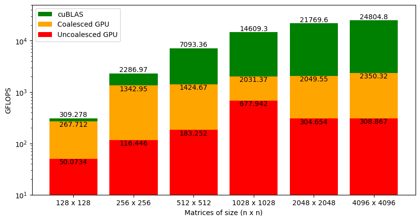
Figure 3.11: cuBLAS vs Coaleased vs Uncoalesced

Figure 3.11 shows the GFLOPS for the coalesced and uncoalesced code against NVIDIA's SGEMM implementation. As we saw earlier, the uncoalesced version achieved 1% of what cuBLAS can do for large matrices. With coalesced memory accesses, the kernel is at 9% of cuBLAS (a big jump from earlier but still insufficient). Interestingly, our code is almost on a level with cuBLAS for smaller matrices (i.e., 128 x 128), and the gap widens as the matrix size increases. This is a clue that will help us improve the performance of our code further. But first, let's see what happens if we use Tensor cores instead of CUDA cores.

Chapter 4: GPU Shared Memory

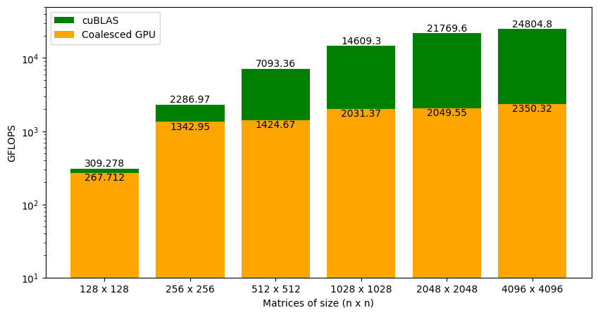
Figure 4.1 shows the performance of the kernel with coalesced memory accesses against cuBLAS SGEMM. For 128 x 128 matrices, the performance is very close. As the matrix size increases, the gap between cuBLAS and our code increases drastically.

The main difference between matrix multiplication involving 128 x 128 matrices and 4096 x 4096 matrices is the amount of data accessed from global memory. As the global memory has long latency and low bandwidth, we need to find a way to reduce global memory accesses or in other words, perform more operations per byte of data accessed from global memory. We need a deeper understanding of the GPU memory hierarchy to do this.

GPU Memory Hierarchy

We already know that GPU is organized as an array of SMs. Programmers never interact with SMs directly. Instead, they use programming constructs like thread and thread blocks to interface with the hardware. When multiple blocks are assigned to an SM, the on-chip memory is divided amongst these blocks hierarchically (see Figure 4.2). Let's now look at the on-chip memory in more detail.

On-chip memory units reside near the cores. Hence, data access from on-chip memory is blazing fast. The issue in this case is that the size of these memory units is very small (maximum of ~16KB per SM). We can manage two main types of on-chip memory units with code.

Shared Memory

Shared memory is a small memory space (~16KB per SM) that resides on-chip and has a short latency with high bandwidth. On a software level, it can only be written and read by the threads within a block.

Registers

Registers are extremely small (~8KB per SM) and extremely fast memory units that reside on-chip. On a software level, it can be written and read by an individual thread (i.e., private to each thread).

💡

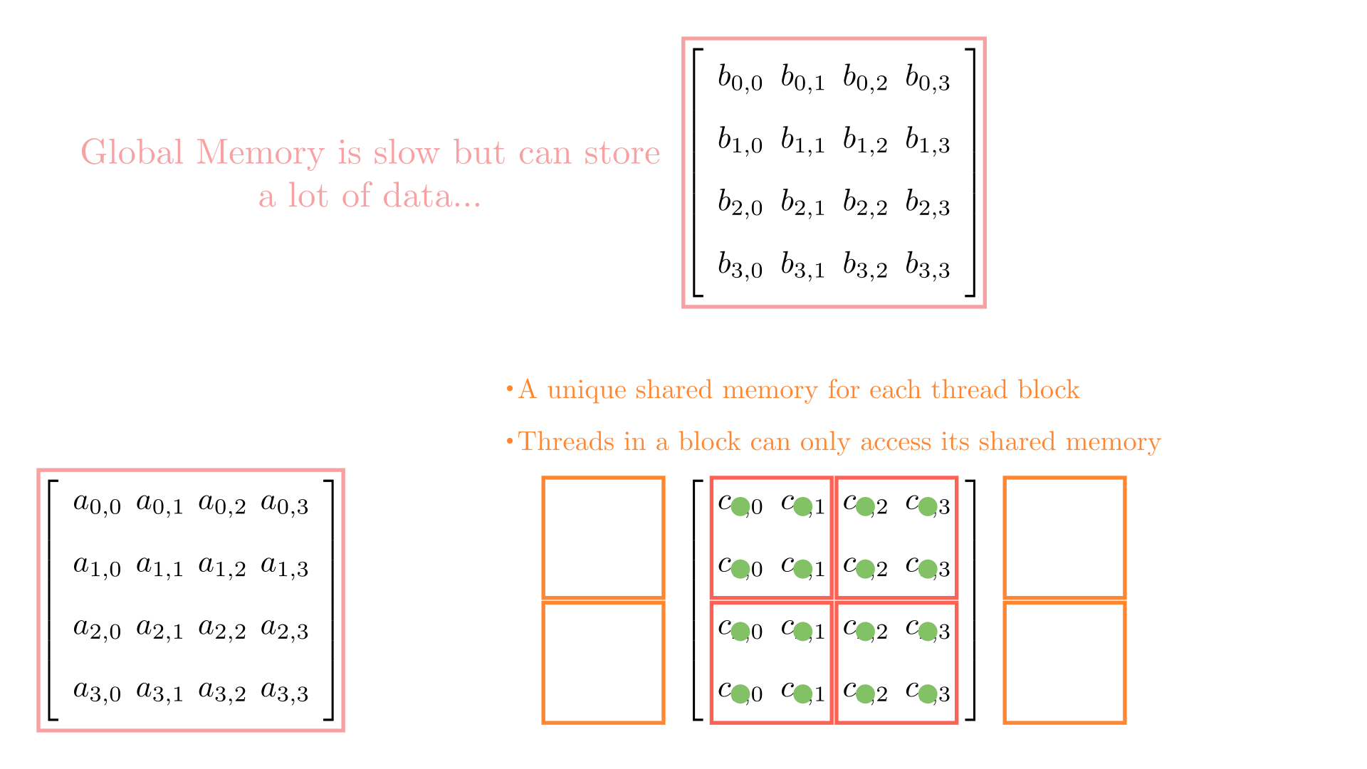
This is in stark contrast to global memory that all threads can access!

To avoid multiple global memory accesses, we can partition the data into subsets called tiles so each tile fits into the shared memory and performs multiple operations on this data. Accessing data from shared memory is fast. This should give a substantial speed up. However, there are two things that we need to keep in mind:

Shared memory is small, so we can only move very small subsets of data to and from shared memory (one at a time).
The correctness of the algorithm should not be affected by this strategy.

Tiled Matrix Multiplication

For simplicity, consider a matrix multiplication involving matrices of size 4. To facilitate parallel computations, let's define a 2 x 2 grid (i.e., 2 blocks each in x and y) and 2 x 2 blocks (i.e., 2 threads each in x and y). Figure 4.3 shows the computations involving all the blocks in the grid.

Figure 4.3: 4x4 matrix multiplication involving 2x2 blocks and 2x2 grid.

Let's see how each thread in this block accesses data from the global memory. As a quick recap, the for loop in the kernel function accesses the elements of A and B, one by one.

for (int k = 0; k < A_n_cols; k++)
{
    value += d_A_ptr[row*A_n_cols + k] * d_B_ptr[k*C_n_cols + col];
}

Figure 4.4 shows the elements accessed by each thread for values of k ranging from 0 to 2.

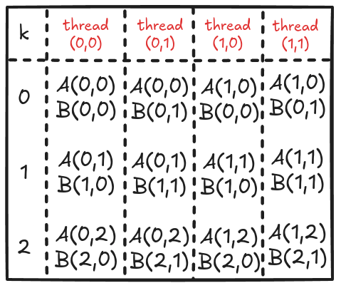
Figure 4.4: Threads and global memory accesses.

Analyzing these memory accesses, we see they are quite inefficient! Just look at k=0; Thread(0,0) and Thread(0,1) both access the same element A(0,0) from global memory. The same can be said for Thread(0,0) and Thread(1,0), where these two are again accessing B[0,0] individually from the global memory. These multiple global memory accesses are costly, and it would be better if we access these elements once, store them in shared memory, and then all threads in a block can use them whenever necessary!

The strategy here is to divide the matrices A and B into tiles of the same shape as the thread block. This is just to keep the code simple. Then, an outer loop (say phase) loops over the tiles (one by one). Inside each phase, each thread in the block loads one element from global to shared memory. Once all the elements are loaded in the shared memory, an inner loop (say k_phase) performs the dot product (just like k in the last kernel function). The catch is that all elements accessed by k_phase are in shared memory, so there's very little cost associated with these memory accesses.

For 4x4 matrices, we will have two phases, and Figure 4.5 shows tiles loading into shared memory in each phase. Each thread is assigned one element, and all threads in a block load these elements into shared memory (in parallel). Once the elements are in the shared memory, matrix multiplication is performed using the data in the shared memory. Each iteration accumulates the result, and the final result can be stored back in the output matrix.

Figure 4.5: Loading tiles into shared memory and performing matrix multiplication in multiple phases

Figure 4.6 shows the elements accessed by each thread for different values of phase (keeping the data in Figure 4.6 consistent with Figure 4.4).

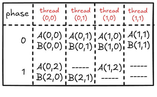
Figure 4.6: Threads and global memory accesses using shared memory

Each thread previously was accessing 6 elements from global memory. Now that has been reduced to 4 or 3 (almost halved). This might not look significant, but remember that we will use this code to perform large matrix multiplications (and not 4x4). It is worth noting that if the tile size is kxk (in the case discussed above, it was 2x2), the global memory traffic will be reduced to 1/k. So, the focus should be to keep the tile size as large as possible (ensuring that it fits in the limited shared memory).

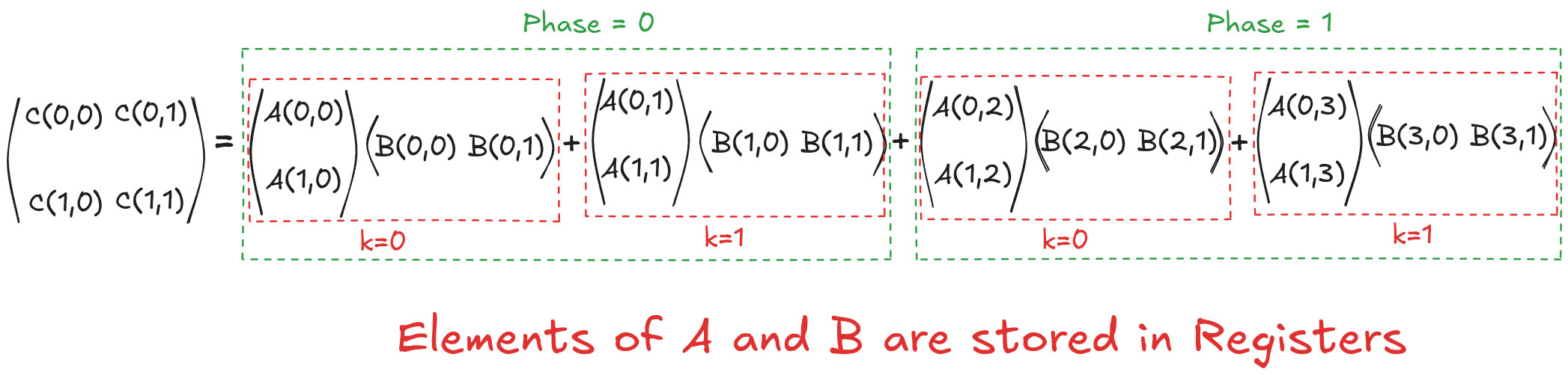
The tiling works because the matrix multiplication algorithm supports it! Algorithmically, we are just splitting one large loop (k) into two smaller loops(phase and k_phase). For example, consider the calculations for computing the output element C[0,0]:

Original Version

$$C[0,0]= \overbrace{A[0,0] \cdot B[0,0]}^{k=0} + \overbrace{A[0,1] \cdot B[1,0]}^{k=1} + \overbrace{A[0,2] \cdot B[2,0]}^{k=2} + \overbrace{A[0,3] \cdot B[3,0]}^{k=3}$$

Tiled Version

$$C[0,0]= \overbrace{\overbrace{A[0,0] \cdot B[0,0]}^{k_{phase}=0} + \overbrace{A[0,1] \cdot B[1,0]}^{k_{phase}=1}}^{phase=0} + \overbrace{\overbrace{A[0,2] \cdot B[2,0]}^{k_{phase}=0} + \overbrace{A[0,3] \cdot B[3,0]}^{k_{phase}=1}}^{phase=1}$$

Writing a kernel function that supports tiling can be a little tricky. However, I will explain everything by dividing the whole process into 8 simple steps:

The first thing we need to do is make sure that the block's dimensions are the same as the tile size. This is just to keep the code simple.

// Ensure that TILE_WIDTH = BLOCK_SIZE
assert(TILE_WIDTH == blockDim.x);
assert(TILE_WIDTH == blockDim.y);

Let's store the block and thread indices in variables and find out the coordinate of the element of C that the select thread will work on. Then, we can also allocate shared memory for A and B.

💡

Remember that automatic variables are private to threads (hence a separate copy for each thread).

// Details regarding this thread
const int by = blockIdx.y;
const int bx = blockIdx.x; 

const int ty = threadIdx.y;
const int tx = threadIdx.x; 

// Working on C[row,col]
const int row = TILE_WIDTH*by + ty;
const int col = TILE_WIDTH*bx + tx;

// Allocating shared memory
__shared__ float sh_A[TILE_WIDTH][TILE_WIDTH];
__shared__ float sh_B[TILE_WIDTH][TILE_WIDTH];

Next, we divide matrices A and B into multiple tiles (or phases) and loop over the tiles one by one.

// Phases
const int phases = ceil((float)A_n_cols/TILE_WIDTH);

// Parallel mat mul
float value = 0;
for (int phase = 0; phase < phases; phase++)
{
    // .
    // .
    // .
}

As the block size is the same as the tile width, each thread is responsible for copying an element from matrices A and B. Figure 4.5 illustrates which thread will copy which element, but here are the key points:
1. For an element of matrix A, the row index is the same as the global index of the thread in the y direction (i.e., row), and the column index is decoded by first deciding which tile number it is (i.e. phase*TILE_WIDTH), and then the local thread index in the x direction (i.e. tx) is added to it (remember that the x index of the thread maps to the columns of A).
2. For an element of matrix B, the row index is decoded by first deciding which tile number it is (i.e. phase*TILE_WIDTH), and then the local thread index in the y direction (i.e. ty) is added to it (remember that the y index of the thread maps to the rows of B), and the column index is the same as the global index of the thread in the x direction (i.e., col).
3. Remember that if a thread does not load a value into shared memory, then that spot in the shared memory must be set to 0 to avoid corruption of the final results.

// Parallel mat mul
float value = 0;
for (int phase = 0; phase < phases; phase++)
{
    // Load Tiles into shared memory
    if ((row < C_n_rows) && ((phase*TILE_WIDTH+tx) < A_n_cols))
      sh_A[ty][tx] = d_A_ptr[(row)*A_n_cols + (phase*TILE_WIDTH+tx)];
    else
      sh_A[ty][tx] = 0.0f;

    if (((phase*TILE_WIDTH + ty) < A_n_cols) && (col < C_n_cols))
      sh_B[ty][tx] = d_B_ptr[(phase*TILE_WIDTH + ty)*C_n_cols + (col)];
    else
      sh_B[ty][tx] = 0.0f;
    
    // .
    // .
    // .
}

The whole point of tiling is that all threads in a block can access all elements (necessary) for their computations. As data copying into shared memory is done in parallel by multiple threads (and it's coalesced), we must ensure the complete tile is loaded before moving forward! This is done using __syncthreads() which holds the code execution (at this point) until all threads have reached there.

// Parallel mat mul
float value = 0;
for (int phase = 0; phase < phases; phase++)
{
    // Load Tiles into shared memory
    if ((row < C_n_rows) && ((phase*TILE_WIDTH+tx) < A_n_cols))
      sh_A[ty][tx] = d_A_ptr[(row)*A_n_cols + (phase*TILE_WIDTH+tx)];
    else
      sh_A[ty][tx] = 0.0f;

    if (((phase*TILE_WIDTH + ty) < A_n_cols) && (col < C_n_cols))
      sh_B[ty][tx] = d_B_ptr[(phase*TILE_WIDTH + ty)*C_n_cols + (col)];
    else
      sh_B[ty][tx] = 0.0f;
    
    // Wait for all threads to load elements
    __syncthreads();

    // .
    // .
    // .
}

Finally, we can perform the dot product using the data loaded into the shared memory.

// Parallel mat mul
float value = 0;
for (int phase = 0; phase < phases; phase++)
{
    // Load Tiles into shared memory
    if ((row < C_n_rows) && ((phase*TILE_WIDTH+tx) < A_n_cols))
      sh_A[ty][tx] = d_A_ptr[(row)*A_n_cols + (phase*TILE_WIDTH+tx)];
    else
      sh_A[ty][tx] = 0.0f;

    if (((phase*TILE_WIDTH + ty) < A_n_cols) && (col < C_n_cols))
      sh_B[ty][tx] = d_B_ptr[(phase*TILE_WIDTH + ty)*C_n_cols + (col)];
    else
      sh_B[ty][tx] = 0.0f;
    __syncthreads();

    // Dot product
    for (int k_phase = 0; k_phase < TILE_WIDTH; k_phase++)
        value += sh_A[ty][k_phase] * sh_B[k_phase][tx];
    
    // .
    // .
    // .
}

As the loop moves to the next iteration, it starts by loading the shared memory with new tiles. For this reason, we must again ensure that all threads have completed their dot product evaluation and avoid data corruption!

// Parallel mat mul
float value = 0;
for (int phase = 0; phase < phases; phase++)
{
    // Load Tiles into shared memory
    if ((row < C_n_rows) && ((phase*TILE_WIDTH+tx) < A_n_cols))
      sh_A[ty][tx] = d_A_ptr[(row)*A_n_cols + (phase*TILE_WIDTH+tx)];
    else
      sh_A[ty][tx] = 0.0f;

    if (((phase*TILE_WIDTH + ty) < A_n_cols) && (col < C_n_cols))
      sh_B[ty][tx] = d_B_ptr[(phase*TILE_WIDTH + ty)*C_n_cols + (col)];
    else
      sh_B[ty][tx] = 0.0f;
    __syncthreads();

    // Dot product
    for (int k_phase = 0; k_phase < TILE_WIDTH; k_phase++)
        value += sh_A[ty][k_phase] * sh_B[k_phase][tx];
    
    // Wait for all threads to finish dot product
    __syncthreads();
}

💡

You might be thinking, how can this tiled version be better because there are two loops? If you look carefully, the two loops are significantly smaller than the one big loop in the standard matrix multiplication kernel. Essentially, we are breaking a single long-running loop into smaller phases (that run faster). This technique is known as strip mining and is not unique to GPU programming.

The last step is to store the calculated value in matrix C. We must ensure that the threads return the results in the valid memory locations.

// Assigning calculated value
if ((row < C_n_rows) && (col < C_n_cols))
    d_C_ptr[(row)*C_n_cols + (col)] =  1*value + 0*d_C_ptr[(row)*C_n_cols + (col)];

Putting all 8 steps together, we have a parallel implementation of tiled matrix multiplication.

__global__ void tiled_mat_mul_kernel(float *d_A_ptr, float *d_B_ptr, float *d_C_ptr, int C_n_rows, int C_n_cols, int A_n_cols)
{
    // Ensure that TILE_WIDTH = BLOCK_SIZE
    assert(TILE_WIDTH == blockDim.x);
    assert(TILE_WIDTH == blockDim.y);
    
    // Details regarding this thread
    const int by = blockIdx.y;
    const int bx = blockIdx.x; 

    const int ty = threadIdx.y;
    const int tx = threadIdx.x; 

    // Working on C[row,col]
    const int row = TILE_WIDTH*by + ty;
    const int col = TILE_WIDTH*bx + tx;

    // Allocating shared memory
    __shared__ float sh_A[TILE_WIDTH][TILE_WIDTH];
    __shared__ float sh_B[TILE_WIDTH][TILE_WIDTH];

    // Phases
    const int phases = ceil((float)A_n_cols/TILE_WIDTH);

    // Parallel mat mul
    float value = 0;
    for (int phase = 0; phase < phases; phase++)
    {
        // Load Tiles into shared memory
        if ((row < C_n_rows) && ((phase*TILE_WIDTH+tx) < A_n_cols))
          sh_A[ty][tx] = d_A_ptr[(row)*A_n_cols + (phase*TILE_WIDTH+tx)];
        else
          sh_A[ty][tx] = 0.0f;

        if (((phase*TILE_WIDTH + ty) < A_n_cols) && (col < C_n_cols))
          sh_B[ty][tx] = d_B_ptr[(phase*TILE_WIDTH + ty)*C_n_cols + (col)];
        else
          sh_B[ty][tx] = 0.0f;
        __syncthreads();

        // Dot product
        for (int k_phase = 0; k_phase < TILE_WIDTH; k_phase++)
            value += sh_A[ty][k_phase] * sh_B[k_phase][tx];
        __syncthreads();
    }
    // Assigning calculated value
    if ((row < C_n_rows) && (col < C_n_cols))
        d_C_ptr[(row)*C_n_cols + (col)] =  1*value + 0*d_C_ptr[(row)*C_n_cols + (col)];
}

Benchmark

Figure 4.7: cuBLAS vs Coaleased vs Shared Memory

Figure 4.7 shows the GFLOPS for the coalesced and shared memory code (where tile size is 32x32) against NVIDIA's SGEMM implementation. As we saw earlier, the coalesced version achieved around 9% of what cuBLAS can do for large matrices. With shared memory accesses, the kernel is at around 12% of cuBLAS. This did not result in a big performance jump. Again, the GFLOPS trend is similar to the coalesced version of the kernel function. Our code is almost on a level with cuBLAS for smaller matrices (i.e., 128 x 128), but the gap widens as the matrix size increases. We will have to analyze this further to understand why this is happening.

Chapter 5: 1D Thread Coarsening using GPU Registers

I want to start this post by briefly analyzing the kernel in step 4 (keeping actual hardware in mind). Compiling the code with flags --ptxas-options=-v outputs that we are using 8192 bytes (8 KB) of shared memory. As I am using 32x32 blocks, there are 1024 threads per block. Below are the specifications for the RTX 3090:

Max Threads per Block: 1024
Max Threads per SM: 1536
Max Shared Memory per Block: 48 KB
Max Shared Memory per SM: 100 KB

As the whole block gets assigned to an SM, the program runs on the hardware as follows:

Shared memory: We are using 8 KB per Block + 1 KB per Block for CUDA runtime usage, resulting in a total of 9 KB per Block.
Threads: We use 1024 Threads per Block, and a maximum of 1536 threads per SM is supported.

This means that our code is running 1 block per SM in parallel at a time. So, in short, a larger portion of the calculations run in sequence. Wouldn't it be better if:

We manually serialize a portion of the code. This way we can avoid the cost of letting hardware handle it automatically and ensure that more blocks get assigned to an SM.
Even though shared memory accesses are not that costly (compared to global memory), can we still reduce the number of shared memory accesses to make the code even faster?

We can achieve both these goals by using a thread to compute multiple elements of the output matrix C and utilize registers wisely (such that memory accesses are even faster).

1D Thread Coarsening

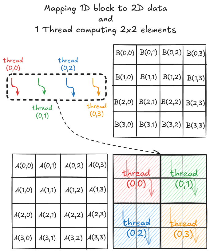
The strategy here is to use a thread to compute multiple elements along the column of the output matrix C. Consider a simple 4x4 matrix multiplication. To solve this in parallel, let's define a 1x1 grid (i.e., 1 block only) and 1x8 block (i.e., 1D block with 8 threads in x direction). Even though the block is 1D, we can still distribute the threads to cover the 2D space (see Figure 5.1).

Figure 5.1: 1 thread computing 2 elements of C along the column.

As before, we load the tiles of matrix A and B into shared memory (in multiple phases). The difference is that a tile of A is 4x2, and a tile of B is 2x4. We still need a 4x4 output but have just 8 threads. Using a 1D block, we can redistribute the threads along 4x2 and 2x4 dimensions, ensuring coalesced global memory accesses (see Figure 5.2).

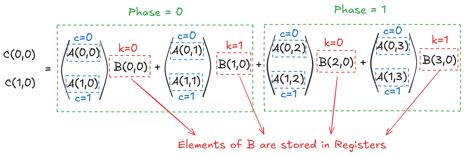
Figure 5.2: Loading tiles into shared memory

Once the tiles are in the shared memory, the kernel in step 4 performs standard matrix multiplication on these tiles. However, in this kernel, 1 thread computes 2 elements. So, we can use registers and store some data to reduce shared memory accesses (remember, the register is private to a thread, so this was not possible in the previous kernels). We will create another loop (call this k) inside each phase. This loop k will retrieve an element of B along the column and store it in a register. Then, a final loop (call this c) calculates the 2 elements of C assigned to the thread using the required elements of A. Figure 5.3 shows the process for Phase 0 (the same thing is done in Phase 1, but with different matrix tiles).

Figure 5.3: Moving elements of B into thread registers

This might look a bit overwhelming, but just consider elements calculated by thread[0,0], i.e., C[0,0] and C[1,0]:

Tiled Version with No Registers

$$C[1,0]= \underbrace{\underbrace{A[1,0] \cdot B[0,0]}_{k_{phase}=0} + \underbrace{A[1,1] \cdot B[1,0]}_{k_{phase}=1}}_{phase=0} + \underbrace{\underbrace{A[1,2] \cdot B[2,0]}_{k_{phase}=0} + \underbrace{A[1,3] \cdot B[3,0]}_{k_{phase}=1}}_{phase=1}$$

Tiled Version with Registers

Now, let's put everything we have discussed into code for general matrix multiplication. Defining grid and block dimensions requires careful analysis now. We must tie the tile sizes and the number of elements each thread computes for compatibility. I decided to go with 64x8 tiles for A and 8x64 tiles for B. Based on this, in my code, each thread computes 8 elements.

// Coalescing Factor
#define COARSE_FACTOR 8

// Tiles of A
#define tiles_A_rows 64
#define tiles_A_cols 8

// Tiles of B
#define tiles_B_cols 64

As each thread in a block copies 1 element from global to shared memory, the block is 1D with 512 threads. As each thread is computing 8 elements along the column of C, a block is assigned to compute 64x64 tile of C. We can use this to define a grid-spanning matrix C.

// Kernel execution
dim3 dim_grid(ceil(C_n_cols/(float)(tiles_B_cols)), ceil(C_n_rows/(float)(tiles_A_rows)));
dim3 dim_block(tiles_A_rows*tiles_B_cols/COARSE_FACTOR);
coarse_1d_mat_mul_kernel<<<dim_grid, dim_block>>>(d_A_ptr, d_B_ptr, d_C_ptr, C_n_rows, C_n_cols, A_n_cols);

💡

As each block has 512 threads and an SM can have a max of 1536 thread, there will be more than 1 block assigned to each SM! This will result in much better latency hiding.

We can now start defining the kernel function. As the block is 1D and threads will get distributed differently (based on what they're doing), we can do the bookkeeping beforehand.

__global__ void coarse_1d_mat_mul_kernel(float *d_A_ptr, float *d_B_ptr, float *d_C_ptr, int C_n_rows, int C_n_cols, int A_n_cols)
{
  // Details regarding this thread
  const int by = blockIdx.y;
  const int bx = blockIdx.x; 

  const int tx = threadIdx.x; 

  // 1D -> 2D while loading A
  const int A_view_ty = tx / tiles_A_cols;
  const int A_view_tx = tx % tiles_A_cols;

  // 1D -> 2D while loading B
  const int B_view_ty = tx / tiles_B_cols;
  const int B_view_tx = tx % tiles_B_cols;

  // Working on C[row,col]
  const int row = tiles_A_rows*by + COARSE_FACTOR * (tx/tiles_B_cols);
  const int col = tiles_B_cols*bx + (tx % tiles_B_cols);

  // .
  // .
  // .
}

The next step is to allocate the shared memory and load tiles of A and B. In this case, the thread-to-element mapping is very similar to before. The only difference is that we must carefully use the block indices and load the correct tiles into shared memory.

__global__ void coarse_1d_mat_mul_kernel(float *d_A_ptr, float *d_B_ptr, float *d_C_ptr, int C_n_rows, int C_n_cols, int A_n_cols)
{
  // Details regarding this thread
  const int by = blockIdx.y;
  const int bx = blockIdx.x; 

  const int tx = threadIdx.x; 

  // 1D -> 2D while loading A
  const int A_view_ty = tx / tiles_A_cols;
  const int A_view_tx = tx % tiles_A_cols;

  // 1D -> 2D while loading B
  const int B_view_ty = tx / tiles_B_cols;
  const int B_view_tx = tx % tiles_B_cols;

  // Working on C[row,col]
  const int row = tiles_A_rows*by + COARSE_FACTOR * (tx/tiles_B_cols);
  const int col = tiles_B_cols*bx + (tx % tiles_B_cols);

  // Allocating shared memory
  __shared__ float sh_A[tiles_A_rows][tiles_A_cols];
  __shared__ float sh_B[tiles_A_cols][tiles_B_cols];

  // Phases
  const int phases = ceil((float)A_n_cols/tiles_A_cols);

  // Parallel mat mul
  float value[COARSE_FACTOR] = {0.0f};
  for (int phase = 0; phase < phases; phase++)
  {
    // Load Tiles into shared memory
    if ((by*tiles_A_rows + A_view_ty < C_n_rows) && ((phase*tiles_A_cols+A_view_tx) < A_n_cols))
      sh_A[A_view_ty][A_view_tx] = d_A_ptr[(by*tiles_A_rows + A_view_ty)*A_n_cols + (phase*tiles_A_cols+A_view_tx)];
    else
      sh_A[A_view_ty][A_view_tx] = 0.0f;
    
    if (((phase*tiles_A_cols + B_view_ty) < A_n_cols) && (bx*tiles_B_cols + B_view_tx < C_n_cols))
      sh_B[B_view_ty][B_view_tx] = d_B_ptr[(phase*tiles_A_cols + B_view_ty)*C_n_cols + (bx*tiles_B_cols + B_view_tx)];
    else
      sh_B[B_view_ty][B_view_tx] = 0.0f;
    __syncthreads();

    // .
    // .
    // .
  }

  // .
  // .
  // .
}

Once the tiles are in shared memory, we define another loop k that puts an element of B into the thread register. Then the final loop can just perform the standard dot product by retrieving elements of A individually. After all the calculations, we just store the results in matrix C.

__global__ void coarse_1d_mat_mul_kernel(float *d_A_ptr, float *d_B_ptr, float *d_C_ptr, int C_n_rows, int C_n_cols, int A_n_cols)
{
  // Details regarding this thread
  const int by = blockIdx.y;
  const int bx = blockIdx.x; 

  const int tx = threadIdx.x; 

  // 1D -> 2D while loading A
  const int A_view_ty = tx / tiles_A_cols;
  const int A_view_tx = tx % tiles_A_cols;

  // 1D -> 2D while loading B
  const int B_view_ty = tx / tiles_B_cols;
  const int B_view_tx = tx % tiles_B_cols;

  // Working on C[row,col]
  const int row = tiles_A_rows*by + COARSE_FACTOR * (tx/tiles_B_cols);
  const int col = tiles_B_cols*bx + (tx % tiles_B_cols);

  // Allocating shared memory
  __shared__ float sh_A[tiles_A_rows][tiles_A_cols];
  __shared__ float sh_B[tiles_A_cols][tiles_B_cols];

  // Phases
  const int phases = ceil((float)A_n_cols/tiles_A_cols);

  // Parallel mat mul
  float value[COARSE_FACTOR] = {0.0f};
  for (int phase = 0; phase < phases; phase++)
  {
    // Load Tiles into shared memory
    if ((by*tiles_A_rows + A_view_ty < C_n_rows) && ((phase*tiles_A_cols+A_view_tx) < A_n_cols))
      sh_A[A_view_ty][A_view_tx] = d_A_ptr[(by*tiles_A_rows + A_view_ty)*A_n_cols + (phase*tiles_A_cols+A_view_tx)];
    else
      sh_A[A_view_ty][A_view_tx] = 0.0f;
    
    if (((phase*tiles_A_cols + B_view_ty) < A_n_cols) && (bx*tiles_B_cols + B_view_tx < C_n_cols))
      sh_B[B_view_ty][B_view_tx] = d_B_ptr[(phase*tiles_A_cols + B_view_ty)*C_n_cols + (bx*tiles_B_cols + B_view_tx)];
    else
      sh_B[B_view_ty][B_view_tx] = 0.0f;
    __syncthreads();

    for (int k = 0; k < tiles_A_cols; k++)
    {
      float B_val_register = sh_B[k][B_view_tx];
      // Dot product
      for (int c = 0; c < COARSE_FACTOR; c++)
        value[c] += sh_A[B_view_ty*COARSE_FACTOR+c][k] * B_val_register;  
    }
    __syncthreads();
  }

💡

Note that we are performing boundary checks at every step, so this is valid for all matrix sizes!

Benchmark

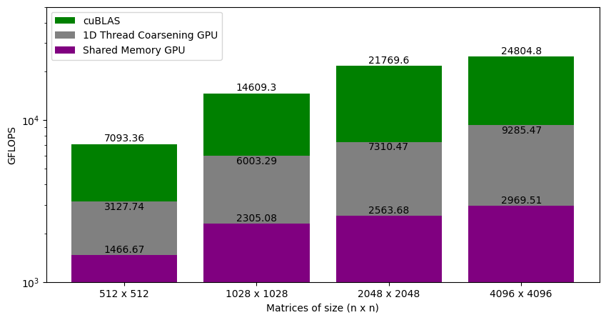
Figure 5.4: cuBLAS vs Shared Memory vs 1D Thread Coarsening

Figure 5.4 shows the GFLOPS for the shared memory code (where tile size is 32x32) and 1D thread coalescing kernel (where each thread computes 8 elements) against NVIDIA's SGEMM implementation. As we saw earlier, the shared memory version achieved around 12% of what cuBLAS can do for large matrices. With 1D thread coarsening, the kernel is at around 37% of cuBLAS. This gives a big performance jump because we are now spending more time performing calculations (and not accessing memory). So, why not keep up and make each thread compute even more elements by storing elements of both A and B in registers?

Chapter 6: 2D Thread Coarsening using GPU Registers

Compiling the code discussed in Chapter 5 with flags --ptxas-options=-v outputs that we are using 4096 bytes (4 KB) of shared memory. That's less than the tiled version discussed in Chapter 4 (which used 8 KB of shared memory). With less shared memory and threads per block, the latency tolerance of the kernel is much better. However, we would still like to reduce the global memory accesses by utilizing the shared memory as much as possible. In this post, I will show how we can enable a thread to compute even more elements of the output matrix C and, in turn, increase the tile sizes of A and B (which will decrease the global memory accesses).

2D Thread Coarsening

The strategy here is very similar to the one discussed in Chapter 5. The difference here is that a thread computes multiple elements along the row and column of the output matrix C. Consider a simple 4x4 matrix multiplication. To solve this in parallel, let's define a 1x1 grid (i.e., 1 block only) and 1x4 block (i.e., 1D block with 4 threads in x direction). Even though the block is 1D, we can still distribute the threads to cover the 2D space (see Figure 6.1).

Figure 6.1: 1 thread computing 4 elements of C along the row and column.

As before, we load tiles of matrix A and B (4x2 and 2x4, respectively). However, we have 4 threads, so filling up the shared memory will take multiple load cycles. Figure 6.2 shows the load cycles for Phase 0 (the process is the same for Phase 1).

Figure 6.2: Loading tiles into shared memory

Once the tiles are in the shared memory, the kernel uses registers and stores the elements of both A and B. Instead of just a single element (as seen in Chapter 5), a small vector of A and B is stored in the thread register. The loop k inside each phase is the same as before, and it decides which row and column vector of A and B, respectively, will be stored in the register. Then, a final two nested loops (call this cy and cx) calculates the 4 elements of C assigned to the thread using the required elements of A and B (in short, this is just the vector cross product). Figure 3 shows the complete process for Phase 0.

Figure 6.3: Moving elements of A and B into thread registers

This might look a bit overwhelming, but just consider elements calculated by thread[0,0], i.e., C[0,0], C[1,0], C[0,1] and C[1,1]:

Tiled Version with No Registers

$$C[0,1]= \underbrace{\underbrace{A[0,0] \cdot B[0,1]}_{k_{phase}=0} + \underbrace{A[0,1] \cdot B[1,1]}_{k_{phase}=1}}_{phase=0} + \underbrace{\underbrace{A[0,2] \cdot B[2,1]}_{k_{phase}=0} + \underbrace{A[0,3] \cdot B[3,1]}_{k_{phase}=1}}_{phase=1}$$

$$C[1,1]= \underbrace{\underbrace{A[1,0] \cdot B[0,1]}_{k_{phase}=0} + \underbrace{A[1,1] \cdot B[1,1]}_{k_{phase}=1}}_{phase=0} + \underbrace{\underbrace{A[1,2] \cdot B[2,1]}_{k_{phase}=0} + \underbrace{A[1,3] \cdot B[3,1]}_{k_{phase}=1}}_{phase=1}$$

Tiled Version with Registers

Now, let's put everything we have discussed into code for general matrix multiplication. Defining grid and block dimensions again requires careful analysis. We must tie the tile sizes and the number of elements each thread computes for compatibility. I decided to go with 128x16 tiles for A and 16x128 tiles for B. Based on this, in my code, each thread computes 8x8 elements.

💡

Note that the tile size is larger than before, so we are utilizing more shared memory.

// Coalescing Factor
#define COARSE_FACTOR_X 8
#define COARSE_FACTOR_Y 8

// Tiles of A
#define tiles_A_rows 128
#define tiles_A_cols 16

// Tiles of B
#define tiles_B_cols 128

Each block is responsible for computing a 128x128 tile of output matrix C, and each thread computes 8x8 elements, so we need a total of 256 threads in a block. We can use this to define a grid-spanning matrix C.

// Kernel execution
dim3 dim_grid(ceil(C_n_cols/(float)(tiles_B_cols)), ceil(C_n_rows/(float)(tiles_A_rows)));
dim3 dim_block(tiles_A_rows*tiles_B_cols/(COARSE_FACTOR_X*COARSE_FACTOR_Y));
coarse_2d_mat_mul_kernel<<<dim_grid, dim_block>>>(d_A_ptr, d_B_ptr, d_C_ptr, C_n_rows, C_n_cols, A_n_cols);

💡

As each block has 256 threads and an SM can have a max of 1536 thread, there will be even more blocks assigned to each SM, resulting in much better latency hiding!

We can now start defining the kernel function. As the block is 1D, threads will get distributed differently (based on their actions). We can do the bookkeeping beforehand and allocate the shared memory. We can also initialize the variables that will store small vectors in registers.

__global__ void coarse_2d_mat_mul_kernel(float *d_A_ptr, float *d_B_ptr, float *d_C_ptr, int C_n_rows, int C_n_cols, int A_n_cols)
{
    // Number of threads per block
    const int n_threads_per_block = tiles_A_rows * tiles_B_cols / (COARSE_FACTOR_X*COARSE_FACTOR_Y);
    static_assert(n_threads_per_block % tiles_A_cols == 0);
    static_assert(n_threads_per_block % tiles_B_cols == 0);

    // Details regarding this thread
    const int by = blockIdx.y;
    const int bx = blockIdx.x; 

    const int tx = threadIdx.x;

    // 1D -> 2D while loading A
    const int A_view_ty = tx / tiles_A_cols;
    const int A_view_tx = tx % tiles_A_cols;
    const int stride_A = n_threads_per_block/tiles_A_cols;

    // 1D -> 2D while loading B
    const int B_view_ty = tx / tiles_B_cols;
    const int B_view_tx = tx % tiles_B_cols;
    const int stride_B = n_threads_per_block/tiles_B_cols;

    // Working on C[row, col]
    const int row = COARSE_FACTOR_Y * (tx / (tiles_B_cols/COARSE_FACTOR_X));
    const int col = COARSE_FACTOR_X * (tx % (tiles_B_cols/COARSE_FACTOR_X));
    
    // Allocating shared memory
    __shared__ float sh_A[tiles_A_rows][tiles_A_cols];
    __shared__ float sh_B[tiles_A_cols][tiles_B_cols];

    // Parallel mat mul
    float value[COARSE_FACTOR_Y][COARSE_FACTOR_X] = {0.0f};
    float register_A[COARSE_FACTOR_X] = {0.0f};
    float register_B[COARSE_FACTOR_Y] = {0.0f};

    // .
    // .
    // .
}

The next step is to load the shared memory with tiles of A and B. The thread-to-element mapping, in this case, is very similar to before. The only difference is that we need multiple iterations to load the correct tiles into shared memory.

__global__ void coarse_2d_mat_mul_kernel(float *d_A_ptr, float *d_B_ptr, float *d_C_ptr, int C_n_rows, int C_n_cols, int A_n_cols)
{
    // Number of threads per block
    const int n_threads_per_block = tiles_A_rows * tiles_B_cols / (COARSE_FACTOR_X*COARSE_FACTOR_Y);
    static_assert(n_threads_per_block % tiles_A_cols == 0);
    static_assert(n_threads_per_block % tiles_B_cols == 0);

    // Details regarding this thread
    const int by = blockIdx.y;
    const int bx = blockIdx.x; 

    const int tx = threadIdx.x;

    // 1D -> 2D while loading A
    const int A_view_ty = tx / tiles_A_cols;
    const int A_view_tx = tx % tiles_A_cols;
    const int stride_A = n_threads_per_block/tiles_A_cols;

    // 1D -> 2D while loading B
    const int B_view_ty = tx / tiles_B_cols;
    const int B_view_tx = tx % tiles_B_cols;
    const int stride_B = n_threads_per_block/tiles_B_cols;

    // Working on C[row, col]
    const int row = COARSE_FACTOR_Y * (tx / (tiles_B_cols/COARSE_FACTOR_X));
    const int col = COARSE_FACTOR_X * (tx % (tiles_B_cols/COARSE_FACTOR_X));
    
    // Allocating shared memory
    __shared__ float sh_A[tiles_A_rows][tiles_A_cols];
    __shared__ float sh_B[tiles_A_cols][tiles_B_cols];

    // Parallel mat mul
    float value[COARSE_FACTOR_Y][COARSE_FACTOR_X] = {0.0f};
    float register_A[COARSE_FACTOR_X] = {0.0f};
    float register_B[COARSE_FACTOR_Y] = {0.0f};

    // Phases
    const int phases = ceil((float)A_n_cols/tiles_A_cols);

    for (int phase = 0; phase < phases; phase++)
    {
        // Load Tiles into shared memory
        for (int load_offset = 0; load_offset < tiles_A_rows; load_offset+=stride_A)
        {
            if ((by*tiles_A_rows + load_offset+A_view_ty < C_n_rows) && ((phase*tiles_A_cols+A_view_tx) < A_n_cols))
                sh_A[load_offset+A_view_ty][A_view_tx] = d_A_ptr[(by*tiles_A_rows+load_offset+A_view_ty)*A_n_cols + (phase*tiles_A_cols+A_view_tx)];
            else
                sh_A[load_offset+A_view_ty][A_view_tx] = 0.0f;
        }
        
        for (int load_offset = 0; load_offset < tiles_A_cols; load_offset+=stride_B)
        {
            if (((phase*tiles_A_cols + B_view_ty+load_offset) < A_n_cols) && (bx*tiles_B_cols + B_view_tx < C_n_cols))
                sh_B[B_view_ty+load_offset][B_view_tx] = d_B_ptr[(phase*tiles_A_cols+B_view_ty+load_offset)*C_n_cols + (bx*tiles_B_cols+B_view_tx)];
            else
                sh_B[B_view_ty+load_offset][B_view_tx] = 0.0f;
        }
        __syncthreads();

        // .
        // .
        // .
    }

    // .
    // .
    // .
}

Once the tiles are in shared memory, inside the loop k, we can populate the registers with sub-vectors of A and B. The final step is to perform cross-product with these vectors (that is done using loops cx and cy). With all the calculations concluded, we can store the results in matrix C.

__global__ void coarse_2d_mat_mul_kernel(float *d_A_ptr, float *d_B_ptr, float *d_C_ptr, int C_n_rows, int C_n_cols, int A_n_cols)
{
    // Number of threads per block
    const int n_threads_per_block = tiles_A_rows * tiles_B_cols / (COARSE_FACTOR_X*COARSE_FACTOR_Y);
    static_assert(n_threads_per_block % tiles_A_cols == 0);
    static_assert(n_threads_per_block % tiles_B_cols == 0);

    // Details regarding this thread
    const int by = blockIdx.y;
    const int bx = blockIdx.x; 

    const int tx = threadIdx.x;

    // 1D -> 2D while loading A
    const int A_view_ty = tx / tiles_A_cols;
    const int A_view_tx = tx % tiles_A_cols;
    const int stride_A = n_threads_per_block/tiles_A_cols;

    // 1D -> 2D while loading B
    const int B_view_ty = tx / tiles_B_cols;
    const int B_view_tx = tx % tiles_B_cols;
    const int stride_B = n_threads_per_block/tiles_B_cols;

    // Working on C[row, col]
    const int row = COARSE_FACTOR_Y * (tx / (tiles_B_cols/COARSE_FACTOR_X));
    const int col = COARSE_FACTOR_X * (tx % (tiles_B_cols/COARSE_FACTOR_X));
    
    // Allocating shared memory
    __shared__ float sh_A[tiles_A_rows][tiles_A_cols];
    __shared__ float sh_B[tiles_A_cols][tiles_B_cols];

    // Parallel mat mul
    float value[COARSE_FACTOR_Y][COARSE_FACTOR_X] = {0.0f};
    float register_A[COARSE_FACTOR_X] = {0.0f};
    float register_B[COARSE_FACTOR_Y] = {0.0f};

    // Phases
    const int phases = ceil((float)A_n_cols/tiles_A_cols);

    for (int phase = 0; phase < phases; phase++)
    {
        // Load Tiles into shared memory
        for (int load_offset = 0; load_offset < tiles_A_rows; load_offset+=stride_A)
        {
            if ((by*tiles_A_rows + load_offset+A_view_ty < C_n_rows) && ((phase*tiles_A_cols+A_view_tx) < A_n_cols))
                sh_A[load_offset+A_view_ty][A_view_tx] = d_A_ptr[(by*tiles_A_rows+load_offset+A_view_ty)*A_n_cols + (phase*tiles_A_cols+A_view_tx)];
            else
                sh_A[load_offset+A_view_ty][A_view_tx] = 0.0f;
        }
        
        for (int load_offset = 0; load_offset < tiles_A_cols; load_offset+=stride_B)
        {
            if (((phase*tiles_A_cols + B_view_ty+load_offset) < A_n_cols) && (bx*tiles_B_cols + B_view_tx < C_n_cols))
                sh_B[B_view_ty+load_offset][B_view_tx] = d_B_ptr[(phase*tiles_A_cols+B_view_ty+load_offset)*C_n_cols + (bx*tiles_B_cols+B_view_tx)];
            else
                sh_B[B_view_ty+load_offset][B_view_tx] = 0.0f;
        }
        __syncthreads();

        // calculate per-thread results
        for (int k = 0; k < tiles_A_cols; ++k) 
        {
            // block into registers
            for (int i = 0; i < COARSE_FACTOR_Y; ++i)
                register_A[i] = sh_A[row+i][k];
            
            for (int i = 0; i < COARSE_FACTOR_X; ++i)
                register_B[i] = sh_B[k][col+i];
            
            for (int cy = 0; cy < COARSE_FACTOR_Y; ++cy) 
            {
                for (int cx = 0; cx < COARSE_FACTOR_X; ++cx) 
                    value[cy][cx] += register_A[cy] * register_B[cx];
            }
        }
        __syncthreads();
    }

    // Assigning calculated value
    for (int cy = 0; cy < COARSE_FACTOR_Y; ++cy)
    {
        for (int cx = 0; cx < COARSE_FACTOR_X; cx++)
        {
            if ((by*tiles_A_rows+row+cy < C_n_rows) && (bx*tiles_B_cols+col+cx < C_n_cols))
                d_C_ptr[(by*tiles_A_rows+row+cy)*C_n_cols + (bx*tiles_B_cols+col+cx)] = 1*value[cy][cx] + 0*d_C_ptr[(by*tiles_A_rows+row+cy)*C_n_cols + (bx*tiles_B_cols+col+cx)];
        }
    } 
}

Benchmark

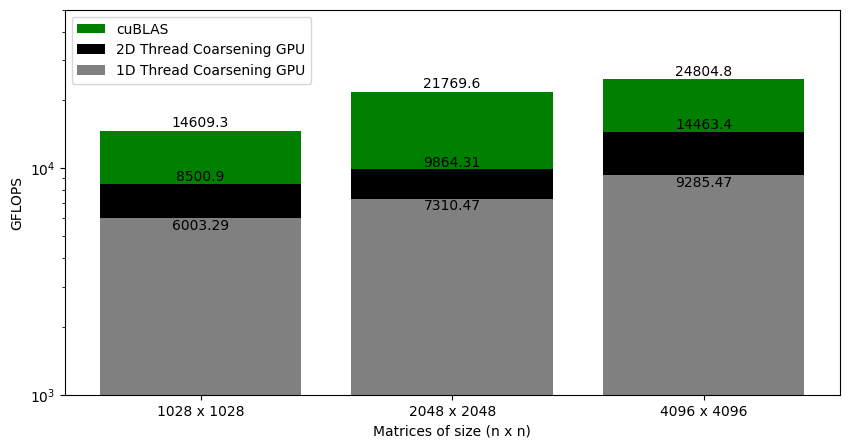
Figure 6.4: cuBLAS vs 1D Thread Coarsening vs 2D Thread Coarsening

Figure 6.4 shows the GFLOPS for the 1D and 2D thread coalescing kernel (where each thread computes 8 and 8x8 elements, respectively) against NVIDIA's SGEMM implementation. As we saw earlier, for the 1D thread coarsening, the kernel was at around 37% of cuBLAS. With 2D thread coarsening, the kernel is at around 58% of the cuBLAS. This gives another big performance jump.

Chapter 7: Vectorized Memory Accesses

Throughout this mini-project, my focus has been on optimizing the memory accesses. It makes sense, as memory is the bottleneck for most applications involving GPUs. In this final blog post, I will show how we can utilize vectorization and speed up the data transfer from global memory to shared memory and shared memory to registers. Vectorization involves using a single processor thread to transfer multiple variables. The catch is that those elements must be next to each other in the memory. For example, consider a task where we need to retrieve four variables ($n_0, n_1, n_2, n_3$). A standard way is to write a loop and access the variables one at a time. If these variables are next to each other in memory (for example, consecutive elements of an array), the compiler will automatically use vectorization and get all the values in a single iteration (Figure 7.1).

💡

When utilizing vectorization, four variables are accessed using a single instruction in parallel.

Figure 7.2 shows the example involving 4x4 matrix multiplication. The strategy here is to use vectorization and access multiple elements of the input matrix A in parallel using a single thread. The 4x2 tile is then stored as a transpose in the shared memory (I will discuss this part shortly). Note that, with vectorization, I don't need multiple iterations to populate the shared memory! The 2x4 tile of the matrix B is accessed similarly. I stored the tile of matrix A as a transpose to again use vectorization and move multiple elements at once into the registers. The same thing is done with the elements of B in the shared memory. Finally, the calculations are performed as usual, and the same thing is repeated for all the other elements of input matrices.

💡

To keep things simple, I'm showcasing parallel access with two elements.

Figure 7.2: Using vectorization to move data between different GPU memory units

The code with vectorized memory accesses is similar to the one in Chapter 6. The first big difference is that the matrix dimensions must also be in multiples of 4.

__global__ void coarse_2d_vec_mat_mul_kernel(float *d_A_ptr, float *d_B_ptr, float *d_C_ptr, int C_n_rows, int C_n_cols, int A_n_cols)
{
    // Number of threads per block
    const int n_threads_per_block = tiles_A_rows * tiles_B_cols / (COARSE_FACTOR_X*COARSE_FACTOR_Y);
    static_assert(n_threads_per_block % tiles_A_cols == 0);
    static_assert(n_threads_per_block % tiles_B_cols == 0);
    static_assert(tiles_A_cols % 4 == 0);
    static_assert(tiles_B_cols % 4 == 0);
    assert(C_n_rows % 4 == 0);
    assert(C_n_cols % 4 == 0);
    assert(A_n_cols % 4 == 0);

    // .
    // .
    // .
}

💡

If the matrices aren't multiples of four, we can always pad them them with zeros.

Everything else is exactly the same until we get to the point where we move data from global to shared memory. This is where we can use float4 and move 4 elements in parallel using a single thread.

__global__ void coarse_2d_vec_mat_mul_kernel(float *d_A_ptr, float *d_B_ptr, float *d_C_ptr, int C_n_rows, int C_n_cols, int A_n_cols)
{
    // Number of threads per block
    const int n_threads_per_block = tiles_A_rows * tiles_B_cols / (COARSE_FACTOR_X*COARSE_FACTOR_Y);
    static_assert(n_threads_per_block % tiles_A_cols == 0);
    static_assert(n_threads_per_block % tiles_B_cols == 0);
    static_assert(tiles_A_cols % 4 == 0);
    static_assert(tiles_B_cols % 4 == 0);
    assert(C_n_rows % 4 == 0);
    assert(C_n_cols % 4 == 0);
    assert(A_n_cols % 4 == 0);

    // Details regarding this thread
    const int by = blockIdx.y;
    const int bx = blockIdx.x; 

    const int tx = threadIdx.x;

    // 1D -> 2D while loading A
    const int A_view_ty = tx / (tiles_A_cols / 4);
    const int A_view_tx = tx % (tiles_A_cols / 4);
    const int stride_A = n_threads_per_block/(tiles_A_cols/4);

    // 1D -> 2D while loading B
    const int B_view_ty = tx / (tiles_B_cols / 4);
    const int B_view_tx = tx % (tiles_B_cols / 4);
    const int stride_B = n_threads_per_block/(tiles_B_cols / 4);

    // Working on C[row, col]
    const int row = COARSE_FACTOR_Y * (tx / (tiles_B_cols/COARSE_FACTOR_X));
    const int col = COARSE_FACTOR_X * (tx % (tiles_B_cols/COARSE_FACTOR_X));
    
    // Allocating shared memory (A is transposed)
    __shared__ float sh_A[tiles_A_cols][tiles_A_rows];
    __shared__ float sh_B[tiles_A_cols][tiles_B_cols];

    // Parallel mat mul
    float value[COARSE_FACTOR_Y][COARSE_FACTOR_X] = {0.0f};
    float register_A[COARSE_FACTOR_X] = {0.0f};
    float register_B[COARSE_FACTOR_Y] = {0.0f};

    // Phases
    const int phases = ceil((float)A_n_cols/tiles_A_cols);

    for (int phase = 0; phase < phases; phase++)
    {
        // Load Tiles into shared memory
        for (int load_offset = 0; load_offset < tiles_A_rows; load_offset+=stride_A)
        {
            if ((by*tiles_A_rows + load_offset+A_view_ty < C_n_rows) && (((phase*tiles_A_cols+A_view_tx*4)) < A_n_cols))
            {
                float4 A_tmp = reinterpret_cast<float4 *>(&d_A_ptr[(by*tiles_A_rows + load_offset+A_view_ty)*A_n_cols + ((phase*tiles_A_cols+A_view_tx*4))])[0];
                sh_A[A_view_tx*4+0][load_offset+A_view_ty] = A_tmp.x;
                sh_A[A_view_tx*4+1][load_offset+A_view_ty] = A_tmp.y;
                sh_A[A_view_tx*4+2][load_offset+A_view_ty] = A_tmp.z;
                sh_A[A_view_tx*4+3][load_offset+A_view_ty] = A_tmp.w;
            }
            else
            {
                sh_A[A_view_tx*4+0][load_offset+A_view_ty] = 0.0f;
                sh_A[A_view_tx*4+1][load_offset+A_view_ty] = 0.0f;
                sh_A[A_view_tx*4+2][load_offset+A_view_ty] = 0.0f;
                sh_A[A_view_tx*4+3][load_offset+A_view_ty] = 0.0f;
            }
            
        }
        
        for (int load_offset = 0; load_offset < tiles_A_cols; load_offset+=stride_B)
        {
            if (((phase*tiles_A_cols + B_view_ty+load_offset) < A_n_cols) && (((bx*tiles_B_cols + B_view_tx*4)) < C_n_cols))
            {
                float4 B_tmp = reinterpret_cast<float4 *>(&d_B_ptr[(phase*tiles_A_cols + B_view_ty+load_offset)*C_n_cols + ((bx*tiles_B_cols + B_view_tx*4))])[0];
                sh_B[B_view_ty+load_offset][B_view_tx*4+0] = B_tmp.x;
                sh_B[B_view_ty+load_offset][B_view_tx*4+1] = B_tmp.y;
                sh_B[B_view_ty+load_offset][B_view_tx*4+2] = B_tmp.z;
                sh_B[B_view_ty+load_offset][B_view_tx*4+3] = B_tmp.w;
            }
            else
            {
                sh_B[B_view_ty+load_offset][B_view_tx*4+0] = 0.0f;
                sh_B[B_view_ty+load_offset][B_view_tx*4+1] = 0.0f;
                sh_B[B_view_ty+load_offset][B_view_tx*4+2] = 0.0f;
                sh_B[B_view_ty+load_offset][B_view_tx*4+3] = 0.0f;
            }
            
        }
        __syncthreads();

        // .
        // .
        // .
    }

    // .
    // .
    // .
}

We don't need to explicitly declare vectorization when moving data from shared memory to registers because the compiler takes care of that. Calculations are performed as usual after the data is loaded in the registers.

__global__ void coarse_2d_vec_mat_mul_kernel(float *d_A_ptr, float *d_B_ptr, float *d_C_ptr, int C_n_rows, int C_n_cols, int A_n_cols)
{
    // Number of threads per block
    const int n_threads_per_block = tiles_A_rows * tiles_B_cols / (COARSE_FACTOR_X*COARSE_FACTOR_Y);
    static_assert(n_threads_per_block % tiles_A_cols == 0);
    static_assert(n_threads_per_block % tiles_B_cols == 0);
    static_assert(tiles_A_cols % 4 == 0);
    static_assert(tiles_B_cols % 4 == 0);
    assert(C_n_rows % 4 == 0);
    assert(C_n_cols % 4 == 0);
    assert(A_n_cols % 4 == 0);

    // Details regarding this thread
    const int by = blockIdx.y;
    const int bx = blockIdx.x; 

    const int tx = threadIdx.x;

    // 1D -> 2D while loading A
    const int A_view_ty = tx / (tiles_A_cols / 4);
    const int A_view_tx = tx % (tiles_A_cols / 4);
    const int stride_A = n_threads_per_block/(tiles_A_cols/4);

    // 1D -> 2D while loading B
    const int B_view_ty = tx / (tiles_B_cols / 4);
    const int B_view_tx = tx % (tiles_B_cols / 4);
    const int stride_B = n_threads_per_block/(tiles_B_cols / 4);

    // Working on C[row, col]
    const int row = COARSE_FACTOR_Y * (tx / (tiles_B_cols/COARSE_FACTOR_X));
    const int col = COARSE_FACTOR_X * (tx % (tiles_B_cols/COARSE_FACTOR_X));
    
    // Allocating shared memory
    __shared__ float sh_A[tiles_A_cols][tiles_A_rows];
    __shared__ float sh_B[tiles_A_cols][tiles_B_cols];

    // Parallel mat mul
    float value[COARSE_FACTOR_Y][COARSE_FACTOR_X] = {0.0f};
    float register_A[COARSE_FACTOR_X] = {0.0f};
    float register_B[COARSE_FACTOR_Y] = {0.0f};

    // Phases
    const int phases = ceil((float)A_n_cols/tiles_A_cols);

    for (int phase = 0; phase < phases; phase++)
    {
        // Load Tiles into shared memory
        for (int load_offset = 0; load_offset < tiles_A_rows; load_offset+=stride_A)
        {
            if ((by*tiles_A_rows + load_offset+A_view_ty < C_n_rows) && (((phase*tiles_A_cols+A_view_tx*4)) < A_n_cols))
            {
                float4 A_tmp = reinterpret_cast<float4 *>(&d_A_ptr[(by*tiles_A_rows + load_offset+A_view_ty)*A_n_cols + ((phase*tiles_A_cols+A_view_tx*4))])[0];
                sh_A[A_view_tx*4+0][load_offset+A_view_ty] = A_tmp.x;
                sh_A[A_view_tx*4+1][load_offset+A_view_ty] = A_tmp.y;
                sh_A[A_view_tx*4+2][load_offset+A_view_ty] = A_tmp.z;
                sh_A[A_view_tx*4+3][load_offset+A_view_ty] = A_tmp.w;
            }
            else
            {
                sh_A[A_view_tx*4+0][load_offset+A_view_ty] = 0.0f;
                sh_A[A_view_tx*4+1][load_offset+A_view_ty] = 0.0f;
                sh_A[A_view_tx*4+2][load_offset+A_view_ty] = 0.0f;
                sh_A[A_view_tx*4+3][load_offset+A_view_ty] = 0.0f;
            }
            
        }
        
        for (int load_offset = 0; load_offset < tiles_A_cols; load_offset+=stride_B)
        {
            if (((phase*tiles_A_cols + B_view_ty+load_offset) < A_n_cols) && (((bx*tiles_B_cols + B_view_tx*4)) < C_n_cols))
            {
                float4 B_tmp = reinterpret_cast<float4 *>(&d_B_ptr[(phase*tiles_A_cols + B_view_ty+load_offset)*C_n_cols + ((bx*tiles_B_cols + B_view_tx*4))])[0];
                sh_B[B_view_ty+load_offset][B_view_tx*4+0] = B_tmp.x;
                sh_B[B_view_ty+load_offset][B_view_tx*4+1] = B_tmp.y;
                sh_B[B_view_ty+load_offset][B_view_tx*4+2] = B_tmp.z;
                sh_B[B_view_ty+load_offset][B_view_tx*4+3] = B_tmp.w;
            }
            else
            {
                sh_B[B_view_ty+load_offset][B_view_tx*4+0] = 0.0f;
                sh_B[B_view_ty+load_offset][B_view_tx*4+1] = 0.0f;
                sh_B[B_view_ty+load_offset][B_view_tx*4+2] = 0.0f;
                sh_B[B_view_ty+load_offset][B_view_tx*4+3] = 0.0f;
            }
            
        }
        __syncthreads();

        // calculate per-thread results
        for (int k = 0; k < tiles_A_cols; ++k) 
        {
            // block into registers
            for (int i = 0; i < COARSE_FACTOR_Y; ++i)
                register_A[i] = sh_A[k][row+i];
            
            for (int i = 0; i < COARSE_FACTOR_X; ++i)
                register_B[i] = sh_B[k][col+i];
            
            for (int cy = 0; cy < COARSE_FACTOR_Y; ++cy) 
            {
                for (int cx = 0; cx < COARSE_FACTOR_X; ++cx) 
                    value[cy][cx] += register_A[cy] * register_B[cx];
            }
        }
        __syncthreads();
    }

    // Assigning calculated value
    for (int cy = 0; cy < COARSE_FACTOR_Y; ++cy)
    {
        for (int cx = 0; cx < COARSE_FACTOR_X; cx++)
        {
            if ((by*tiles_A_rows+row+cy < C_n_rows) && (bx*tiles_B_cols+col+cx < C_n_cols))
                d_C_ptr[(by*tiles_A_rows+row+cy)*C_n_cols + (bx*tiles_B_cols+col+cx)] = 1*value[cy][cx] + 0*d_C_ptr[(by*tiles_A_rows+row+cy)*C_n_cols + (bx*tiles_B_cols+col+cx)];
        }
    } 
}

Benchmark

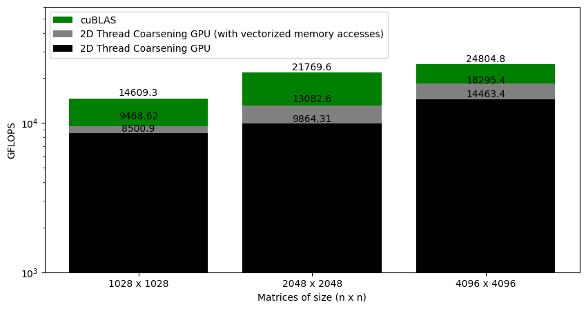
Figure 7.3: cuBLAS vs 2D Thread Coarsening vs 2D Thread Coarsening (with vectorized memory accesses)

With vectorized memory accesses, we got a decent increase in performance, and now the code is at around 70% of cuBLAS performance. There is still some room left for improvement, but that's a topic for the future.

References

YouTube video

Code repository

Blog post by Simon Boehm

Chapter 1: What is SGeMM

Matrices and Computer Memory

Memory Precision

MatrixFP32

Matrix Multiplication

Chapter 2: Getting Started with CUDA Programming

CPU and GPU

GPU Programming Model

Parallel Matrix Multiplication

Benchmark

Chapter 3: GPU Global Memory Coalescing

Modern GPU Architecture

Thread Blocks and SMs

Warps

Kernel Function

Answering the Questions

Why does GFLOPS increase with increasing Matrix Size?

How to improve Kernel Performance?

Benchmark

Chapter 4: GPU Shared Memory

GPU Memory Hierarchy

Tiled Matrix Multiplication

Benchmark

Chapter 5: 1D Thread Coarsening using GPU Registers

1D Thread Coarsening

Benchmark

Chapter 6: 2D Thread Coarsening using GPU Registers

2D Thread Coarsening

Benchmark

Chapter 7: Vectorized Memory Accesses

Benchmark

References

Subscribe to 0Mean1Sigma