By Tushar Gautam in GPU Programming — Nov 28, 2024

What is SGeMM

SGeMM stands for Single-Precision General Matrix Multiplication. Let's analyze matrix multiplication on a CPU and a GPU.

Photo by Enric Moreu / Unsplash

Introduction

SGeMM stands for Single-Precision General Matrix Multiplication. Matrix is a rectangular array of numbers arranged in rows and columns. So, an M by N matrix (written as M x N) has M rows and N columns with a total of M x N numbers. Benefit of arranging numbers in a matrix is that it gives structure to the data and we can easily access any number by specifying it's location.

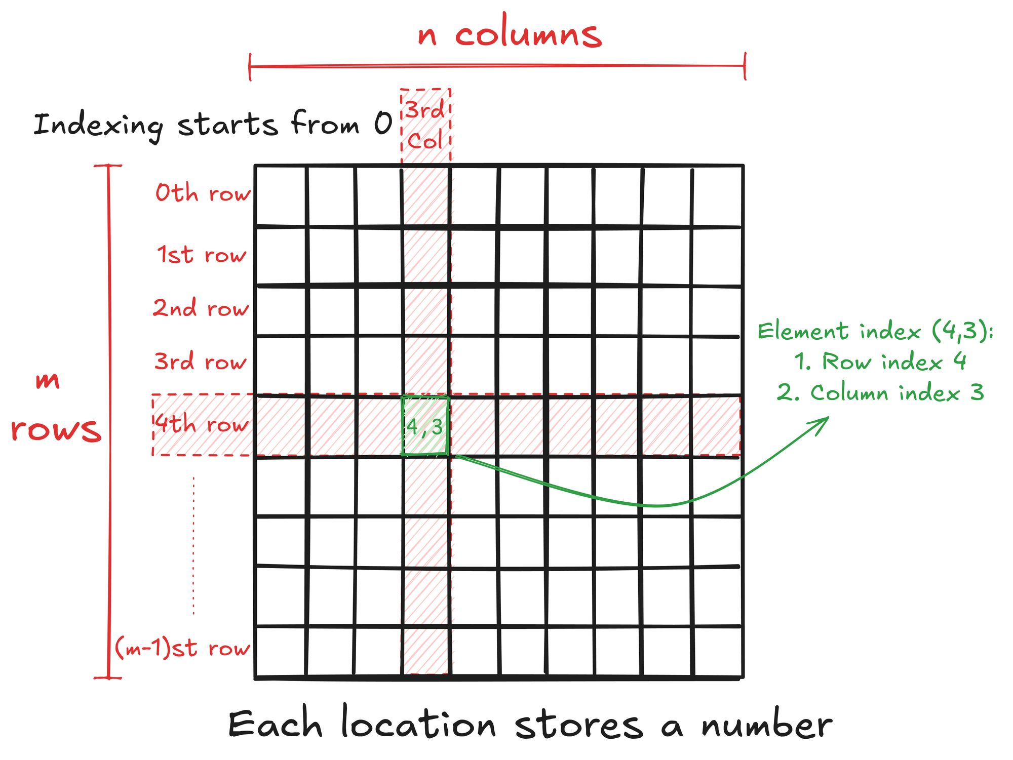
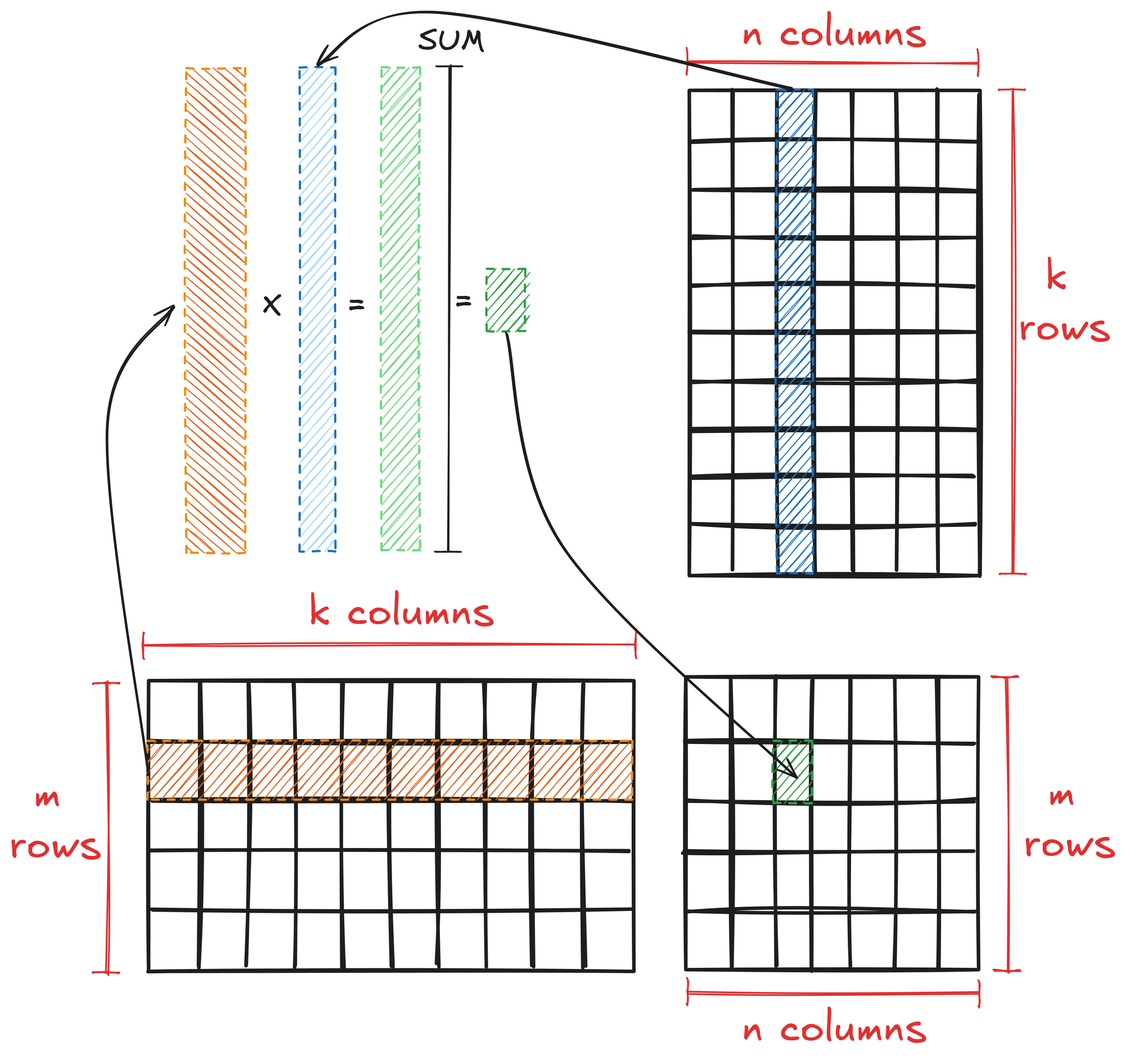
General matrix multiplication is a fundamental operation in linear algebra with specific rules and properties. Matrix multiplication is defined for two matrices A and B only when the number of columns in A is equal to the number of rows in B, i.e., if :

A is an M x K matrix
B is an K x N matrix
Then their product AB is an M x N matrix.

To multiply matrices A and B:

Take each row of A and perform element-wise multiplication of it with each column of B.
The resulting elements are the sum of these multiplications.

Mathematically, this is expressed as:

\( \textbf{AB}_{ij} = \sum_{k=0}^{K-1} \textbf{A}_{i,k} \cdot \textbf{B}_{k,j} \)

Where \(\textbf{AB}_{ij}\) is the element in the i-th row and j-th column of the resulting matrix.

💡

Figure 2 shows how an element of output matrix is computed using a row and a column from input matrices. The same thing is done for all the other elements and only the row and column from the input matrices change.

Matrices and Computer Memory

Computer memory is often presented as a linear address space through memory management techniques. This means that we cannot store a matrix in 2D form. Languages like C/C++ and Python store 2D array of elements in row major layout, i.e., in the memory, 1st row is placed after 0th row, 2nd row after 1st row, and so on.

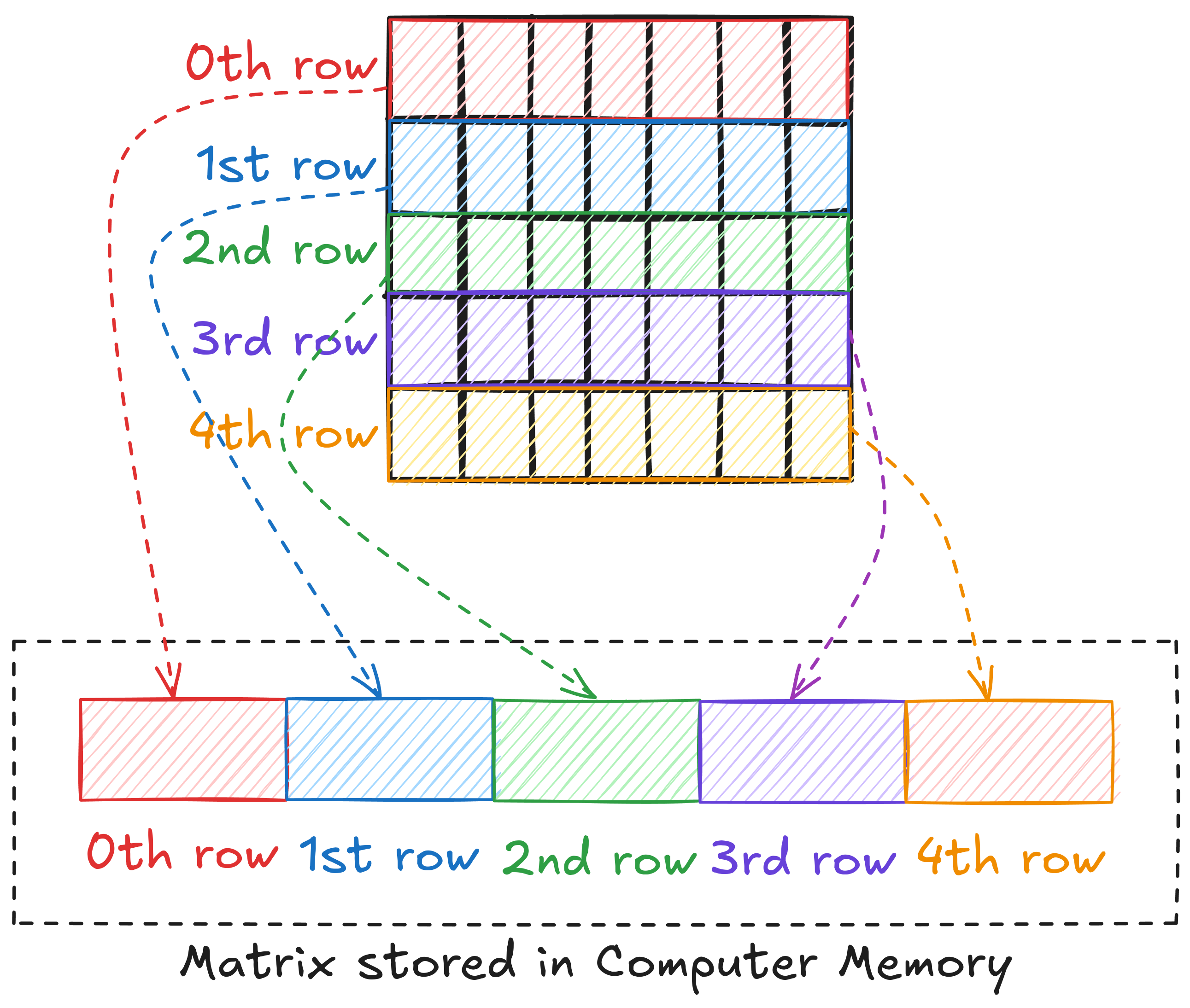
Figure 3: Row major layout for storing matrices

💡

FORTRAN stores 2D arrays in column major layout.

This means that to access an element, we need to linear the 2D index of the element. For example, if matrix A is M x N, then the linearlized index of element (6, 8) can be written as \(6 \cdot N + 8\).

💡

Generally speaking, any element \((i, j)\) is at the location \(i \cdot N + j\) in the memory.

So far, we have discussed matrices in general and the multiplication involving two matrices. Let's now look at what single-precision means.

Memory Precision

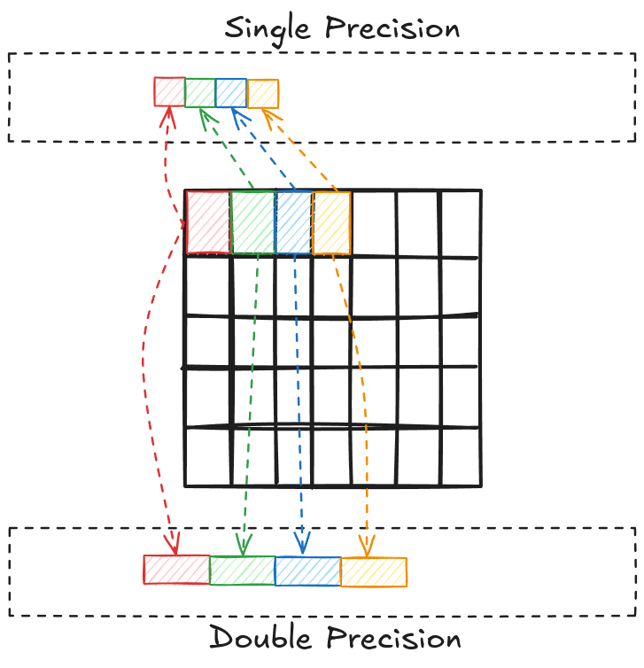
The bit (binary digit) is the smallest and most fundamental unit of digital information and computer memory. A byte is composed of 8 bits and is the most common unit of storage and one of the smallest addressable units of memory in most computer architectures. There are several ways to store the numbers in a matrix. Most common one is known as double precision (declared as double in C/C++). In double precision, a number is stored using 8 consecutive bytes in the memory. Another way is to store the numbers as a single precision type (declared as float in C/C++), where a number is stored using 4 consecutive bytes in the memory. This way we can store the same number that takes up less space in memory, but we give up accuracy and the range of values that we can work with.

💡

Single precision provides about 7 decimal digits of precision, and double precision provides about 15-17 decimal digits of precision. Single precision can represent numbers from approximately \(1.4 \times 10^{-45}\) to \(3.4 \times 10^{38}\), and double precision can represent numbers from approximately \(4.9 \times 10^{-324}\) to \(1.8 \times 10^{308}\).

Single precision is used by NVIDIA because it is generally preferred over double precision on GPUs for a few reasons:

Sufficient accuracy: For many graphics and some scientific computing applications, single precision provides adequate accuracy while offering performance benefits.
Memory bandwidth: Single precision (4-bytes) values require half the memory bandwidth of double precision (8-bytes) values. This allows more data to be transferred between memory and processing units in the same amount of time.
Computational units: GPUs typically have more single precision computational units than double precision units. For example, NVIDIA GPUs often have 2-3x more single precision CUDA cores compared to double precision cores.
Throughput: Single precision operations can be performed at a higher rate than double precision operations. Many GPUs have significantly higher theoretical peak performance for single precision (measured in FLOPS) compared to double precision.
Memory capacity: Using single precision allows more data to fit in the GPU's memory, reducing the need for data transfers between GPU and CPU memory.
Power efficiency: Single precision computations generally consume less power than double precision, allowing for better performance within thermal constraints.
Specialized hardware: Many GPUs have tensor cores or other specialized units optimized for single precision or lower precision (e.g. half precision) calculations, particularly for AI/ML workloads.

💡

Half precision (2-bytes) floating point numbers are not natively supported in standard C++. However, we have an option to use half precision in CUDA (declared as half).

MatrixFP32

Matrix width is essential when linearizing a 2D index of an element. To avoid any mistakes (or confusion) while working with multiple matrices, I defined a simple (lightweight) class MatrixFP32, that keeps track of the float data pointer and the rows/columns of the matrix.

class MatrixFP32
{
public:
    const int n_rows;        // Number of rows
    const int n_cols;        // Number of cols

    // Pointer to dynamic array
    float* ptr;

    // Constructor to initialize n_rows x n_cols matrix
    MatrixFP32(int n_rows, int n_cols);
    
    // Free memory
    void free_mat();
};

MatrixFP32::MatrixFP32(int n_rows_, int n_cols_) : n_rows(n_rows_), n_cols(n_cols_)
{
    // Initialize dynamic array
    ptr = new float[n_rows*n_cols];
}

void MatrixFP32::free_mat()
{
    delete[] ptr;
}

This way I can easily access any element of a matrix defined using MatrixFP32.

// Define an n x n matrix A_FP32
MatrixFP32 A_FP32 = MatrixFP32(n, n);

// Get element (4, 6)
float element = A_FP32.ptr[4*A_FP32.n_cols + 6];

Matrix Multiplication

The algorithm shown in Figure 2 can be written in C++ quite easily (in around 10 lines of code).

void cpu_xgemm(MatrixFP32 A_mat, MatrixFP32 B_mat, MatrixFP32 C_mat)
{
    // Getting A Matrix Dimension
    int A_n_rows = A_mat.n_rows; 
    int A_n_cols = A_mat.n_cols;

    // Getting B Matrix Dimension
    int B_n_rows = B_mat.n_rows; 
    int B_n_cols = B_mat.n_cols;

    // Getting C Matrix Dimension
    int C_n_rows = C_mat.n_rows; 
    int C_n_cols = C_mat.n_cols;

    // Asserting dimensions
    assert (A_n_cols == B_n_rows && "Matrices A & B must have one common dimension");
    assert (A_n_rows == C_n_rows && "A rows must be equal to C rows");
    assert (B_n_cols == C_n_cols && "B cols must be equal to C cols");

    // Matrix Multiplication
    for (int row = 0; row < A_n_rows; row++)
    {
        for (int col = 0; col < B_n_cols; col++)
        {
            float val = 0.0f;
            for (int k = 0; k < A_n_cols; k++)
            {
                val += A_mat.ptr[row*A_n_cols + k] * B_mat.ptr[k*B_n_cols + col];
            }
            C_mat.ptr[row*C_n_cols + col] = val;
        }
    }
}

Sequential matrix multiplication on a CPU

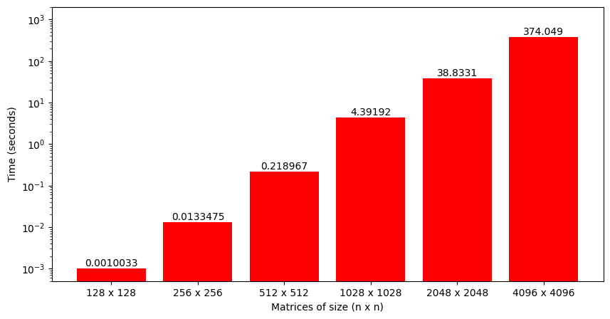
By just looking at this code, we can sense that the algorithm might be computationally intensive (there are 3 nested loops!). Figure 5 plots the time taken to perform matrix multiplication using this code for matrix sizes ranging from 128 to 4096. We can see that the growth is somewhat exponential as the matrix size increases (technically it's around \(n^3\)).

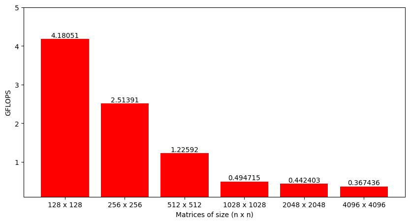
Figure 5: Runtime for sequential matrix multiplications on a CPU

💡

With 1024x increase in the number of elements (from 128 x 128 to 4096 x 4096), execution time increases 3728186x!

Even though time is a perfectly fine metric to analyze, a better option is to look at the number of operations performed per second by the function or Giga Floating-Point Operations per seconds (GFLOPS). When multiplying two matrices of size M x K and K x N, each element of the output matrix requires approximately K multiplications and K additions, i.e. 2K operations. As there are total M x N output elements, the total number of operations are 2 x M x N x K. Dividing this number by the time it took to perform matrix multiplication gives FLOPS for the implemented algorithm (that can be converted to GFLOPS).

Figure 6: GFLOPS for sequential matrix multiplications on a CPU

💡

Figures 5 and 6 show the same thing essentially, but GFLOPS is a more general metric that takes algorithm complexity into account as well and I will be using this moving forward.

Fortunately, matrix multiplication can be parallelized quite efficiently. The next step is to understand how this algorithm can be parallelized and then implement a basic parallel matrix multiplication that runs on the GPU.

To get a taste of the power of GPUs, CUDA provides a function SGEMM that can do this in a single line of code. To be more precise, SGEMM function performs \(C = \alpha A \cdot B + \beta C\) (i.e., matrix multiplication and accumulation). However, we can set \(\alpha=1\) and \(\beta=0\) to just get matrix multiplication.

// Perform matrix multiplication: C = A * B 
float alpha = 1;
float beta = 0;
cublas_check(cublasSgemm(handle,
                        CUBLAS_OP_N, CUBLAS_OP_N,
                        d_C_FP32.n_cols, d_C_FP32.n_rows, d_A_FP32.n_cols, // Num Cols of C, Num rows of C, Shared dim of A and B
                        &alpha,
                        d_B_FP32.ptr, d_B_FP32.n_cols, // Num cols of B
                        d_A_FP32.ptr, d_A_FP32.n_cols, // Num cols of A
                        &beta,
                        d_C_FP32.ptr, d_C_FP32.n_cols) // Num cols of C
            );

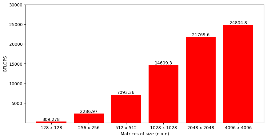
Figure 7: GFLOPS for parallel matrix multiplications on a GPU using cuBLAS

Figure 7 shows the GFLOPS for different matrix sizes, and it's interesting to see that the performance increases as the matrices get larger. This is counter intuitive and, we'll see exactly why this happens.

References

class MatrixFP32

Benchmarking cuBLAS SGEMM